Complex Discrete Systems Graph Simulation

Kadirova, Delovar; Kadirova, Aziza

doi:10.9717/JMIS.2015.2.3.263

J Multimed Inf Syst 2(3):263-274

eISSN: 2383-7632

DOI: https://doi.org/10.9717/JMIS.2015.2.3.263

Section A

Complex Discrete Systems Graph Simulation

Delovar Kadirova¹^,^*, Aziza Kadirova²

Author Information & Copyright ▼

¹Department of EEA, Tashkent State Technical University, Uzbekistan, info@innovation.uz

²Center for Strategic Innovations and Informatization, Uzbekistan, aziza.kaa@mail.ru

^*Corresponding Author: Delovar Kadirova, University str. 2, Tashkent, 100095, Republic of Uzbekistan, info@innovation.uz

© Copyright 2015 Korea Multimedia Society. This is an Open-Access article distributed under the terms of the Creative Commons Attribution Non-Commercial License (http://creativecommons.org/licenses/by-nc/4.0/) which permits unrestricted non-commercial use, distribution, and reproduction in any medium, provided the original work is properly cited.

Received: Aug 11, 2015 ; Revised: Oct 20, 2015 ; Accepted: Nov 02, 2015

Published Online: Sep 30, 2015

Abstract

The subject of this work is the complex discrete systems simulation special features with the aid of dynamic graph models. The proposed simulation technique allows to determine the ways for tasks solutions in terms of discrete systems analysis and synthesis of various complication: one-dimensional and multidimensional, steady and unstable, with the pulse elements abnormal operating mode and others. Often complex control systems analysis and synthesis task solutions, via classical approach comes out to be insolvent, because of the computational problems. The application of graph models allows to perform clear and strict characterization and computer procedures automation. The optimal controls synthesis algorithm presented in this paper, transferring the discrete system from target initial state to target final state within the minimum time, allows to consider the zero initial conditions systems, with the initial potential energy, with the control actions limitations and complex pulse elements operating mode.

Keywords: complex discrete system; dynamic graph model; state variables; synthesis

I. INTRODUCTION

The growing control systems complexity set new problems, connected with

structural properties to be explored;
need to systematize the mathematical formulation of various physical nature elements;
analysis technique unification, as well as analysis and synthesis;
need to jump over the computational problems;
aspiration for maximal clearness and simplicity.

The special value it has in terms for discrete automatic control systems. Here is the presence of dozens pulse elements, that operate according to various linear and non-linear laws, multiple connection, lending variety and complexity to the process structures [1, 2, 5-7].

At the heart of discrete systems mathematical tools are posited the lattice functions, finite differences and sums, linear and non-linear finite-difference equations.

Moreover, in classical works much attention was given to the problems of «close up» some aspects continuous and discrete systems theory. In particularly, such related to some certain works, covering the discrete systems analysis and synthesis frequency methods, Laplace transformation and Laplace discrete transformation as well as other aspects [1, 2, 5, 6, 8-10].

The graph models application is compared favourably in terms of its simplicity as well as availability of huge awareness. Showing the system in more detailed, compared to structural diagram, it holds the visual presentation in terms of signal trip over the system. That simplifies not just the transfer function definition, but demonstrates the influence of any parameter on it, gives a chance to obtain the variety possible structures and practical recommendations in terms of explicit structures decision to implement the necessary connections to system [4, 11].

Should be noted, that the most of works on graphs application cover the problems in static formulation. Unlike the current methods in this paper were demonstrated the dynamic graphs application state variables graphs category and pulse flow graphs, as well as hybrid graphs for complex discrete systems simulation.

II. MODELING METHOD

Let’s consider the linear fixed system l-order, described across the switching intervals by vector-matrix differential formula

x ˙ → (λ) = A → x → (λ) + B → u → (λ),

(1)

where λ = t − jT ; 0 < λ ≤ T

$x → (λ) − (l × 1)$ vector of process state variable (control object) with coordinates x₁,x₂,…x_l;

$u → (λ) − (N × 1)$ vector of input state variable with the coordinates u₁,u₂,…u_N;

$A → − (l × l)$ coefficients matrix real constant;

$B → − (l × N)$ control matrix real constant.

Applying the definition «expanded dimensionality system», the formula (1) will be redrafted as [1]:

v ˙ → (λ) = A → v → (λ),

(2)

where $v → (λ) = [u → (λ) x → (λ)] − (n × 1)$ expanded dimensionality state vector with the coordinates u₁,u₂,…,u_N; x₁,x₂,…,x_l (n = N + l);

$A → − (n × n)$ expanded dimensionality system coefficient matrix.

Equation of state (2) describes the system behavior within the intervals between the switching moments, state variables varying within the pulse elements closure moments characterizes by the transient state formulas:

V → (j T +) = B → v → (j T) .

(3)

The solution of differential equation (2) will write as

V → (λ) = Φ → (λ) V → (0 +),

(4)

where the expanded transition matrix may be defined through the model discussion in state variables or for the general cases from expressions:

Φ → (λ) = L − 1 {p J → − A →} − 1,

(5)

Φ → (λ) = e A → λ .

(6)

Here $Φ → (λ) − (n × n)$ matrix with the coordinates a_ij(λ), that in the event of time-invariant systems present as the constant values, or depending on time for non-stationary systems.

System coordinate values at the pulse element closure moments shall be defined according to recursion

V → (j + 1 ¯ T) = Φ → (T) ⋅ B → ⋅ V → (j T)

(7)

o r V → (j + 1 ¯ T) = H → (T) V → (j T) .

(8)

Have noticed, that in major cases the matrixes $Φ →, B → and H →$ carry a big number of nulls, i.e. come as low of density. Therefore, direct application of formulas (7) or (8) even for the easiest discrete systems, lead to perform overmuch operations.

2.1. State Variables Graphs

Handling redundant information may be excluded if to apply the state variables graphs.

State Variables Graph (SVG) shall mean the oriented weighted graph G(V,Г), vertex set of which V =U(λ)∪X(λ), where U(λ)− is the subset, conform to input variables; X(λ)− subset, conform to control object sate variables; Г - function V in V.

Each graph edge connected to figure (function), named as branch emission t_ik. Each state point (node) holds connected with that variable, called as the main signal x_i.

Emission a_ij graph is equal to signal ratio, arising in j dependent node, to signal i dependent source. The emission a_ij is the matrix $Φ → (λ)$ element and shall be defined according to SVG based on Mezon formula [3]

a i j = x j x i = [(P 1 + P 2 + ... + P n) (1 − L 1) (1 − L 2) ... (1 − L m)] * [(1 − L 1) (1 − L 2) ... (1 − L m)] *,

where P – graph process emission, L– back loop of a graph emission, * – shall mean: «omit terms, containing the products, related to back loops and processes, related to between themselves loops».

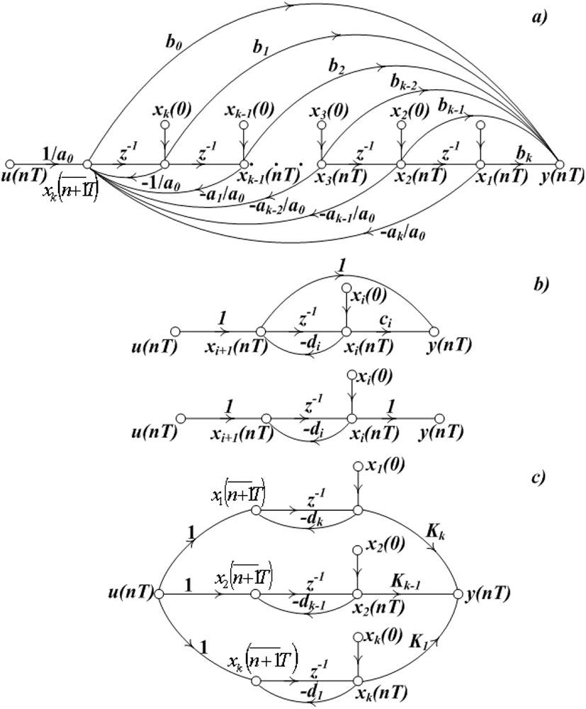
In accordance with the type, wherein has been given transfer function, shall be selected graph creation model (Figure 1).

Fig. 1. SVG, constructed with the aid of machine-level-programming (a), cascade programming (b), and parallel programming (c)

Download Original Figure

2.2. Pulse Flow Graphs

In section 2.1 has been demonstrated the discrete control systems simulation on the basis of state variables graphs application. The SVG application assumes the control object mathematical model availability of the form of differential equations. Moreover, frequently the control objects mathematical models preset with the aid of pulse transient functions.

The pulse transient functions may be defined either based on experiment or formula

A (t) = L − 1 {A (p)},

(9)

With the control object known pulse transient function as well as zero initial conditions it is reasonable to make use the Pulse Flow Graphs (PFG).

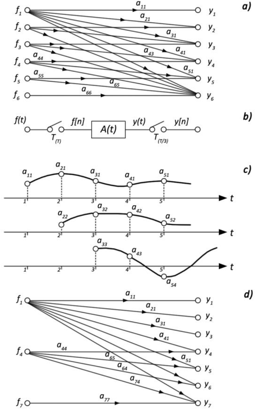
Assume, there was given relation Q = (G,F,Y), where F, Y – some dynasets, G – standardization curve. Will impose on standardization curve G a restriction:

i f i ≥ j, t h e n (f i, y i) ∈ G .

(10)

Further assign to each pair (f_i, y_i) the coefficient a_ij. Assume, that the departure unit element f_i ∊ F shall be compared with the element y_i ∊ Y of arrival domain with the weight a_ij. The present match weighted graph Q = (G,F,Y), in case of, that the dynamic set F comes as the subsequence of short-period impulse signals type of δ = (t) and a_ij – represents the impulse transient system function coefficients, and define the Dynamic Graph Model (DGM) of elemental disconnect process of automatic control discrete system (ACDS).

For illustration, assume F = (f₁,f₂,f₃,f₄,f₅,f₆,), Y = (y₁,y₂,y₃,y₄,y₅,y₆,), then considering (10) will obtain

G = {(f 1, y 1), (f 1, y 2), (f 1, y 3), (f 1, y 4), (f 1, y 5), (f 1, y 6); (f 2, y 2), (f 2, y 3), (f 2, y 4), (f 2, y 5), (f 2, y 6); (f 4, y 4), (f 4, y 5), (f 4, y 6); (f 5, y 5), (f 5, y 6); (f 6, y 6)} .

Assign to each pair (f_i, y_i) the impulse transient function coefficient a_ij. Finally, will obtain DGM the elemental ACDS (Figure 2). In the Figure 2c was explained the accepted coefficients selection and coefficients identification method with pulse transient function for non-steady system continuous part case.

Fig. 2. DGM elemental ACDS

Download Original Figure

Through the rules, specified for signal flow graphs, based on DGM, one may find the process discrete values.

2.3. The Hybrid Graph Models

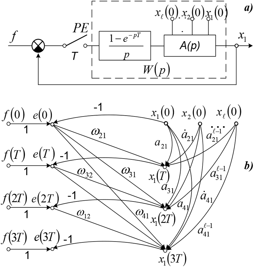
The pulse flow graphs have been defined as the models are very suitable for zero initial conditions systems. Let’s consider the availability based on that the models, enabling to consider the initial potential energy.

Assume we have system l-order, demonstrated in Figure 3a. The pulse flow graph makes the relation between the input coordinate f and coordinate output x₁ system to discrete moments. When are the initial conditions x₁(0),x₂(0),…,x_l(0), then for its record is just enough according to object state variables graph to find the emissions from these coordinates to coordinate output, i.e.

∇ (x 1 (0), x 1 (T)), ∇ (x 2 (0), x 2 (T)), ..., ∇ (x l (0), x l (T))

Fig. 3. HGM of discrete system of l-st order

Download Original Figure

Such emissions have the meaning of pulse transient function and its derivatives, including (l-1)-st derivative. It is necessary to do these functions coefficients sample capture with the required sampling interval and do totalize the signals from points x₁(0),x₂(0),…,x_l(0), with the system signals, caused by action input. Then according to graph model one may define the system processes with nonzero initial conditions (Figure 3b).

Since the similarly models combine with the pulse flow graph and state variables graph properties, they called as Hybrid Graph Models (HGM). The hybrid graph models are comfortable for processes calculation within the systems with delay, pulse elements complex operating modes, when synthesis of optimum in terms of discrete systems operation speed.

The hybrid models application is in fact reasonably for initial potential energy systems, if required the information regarding the behavior of just coordinate output, and the intermediate coordinates are not of interest, or when the performance of synthesis task, when half of coordinates are available for measurement.

Let’s consider the graph models construction principles for discrete systems various classes.

III. THE GRAPH MODELS OF DISCRETE SYSTEMS

3.1. Step-in Phase Systems

Will start consideration from SVG for in step-in phase systems. To describe the transients within discrete systems, account must be taken of pulse elements availability (PE) as well as its operating mode. The discrete system behavior between pulse element switching moments describes by differential formulas modes as follows:

(b l p l + b l − 1 p l − 1 + ... + b 1 p + b 0) y = = (a m p m + a m − 1 p m − 1 + ... + a 1 p + a 0) u,

(11)

Where y – system signal output; u – signal input or system control signal; a_j(j ∊ J = {0,1,2,…,m}) – fixed polynom factors A(p); b_j(i ∊ I = {0,1,2,…,l}) – fixed polynom factors B(p).

Within the switching moments the state variables change shall be described by the formula (3). In state variables graph this will be presented as an incorporation of complementary groups {u(0)},{x(0)} and branches with b_ij emissions, to join its indicated nodes with the initial conditions nodes {u(0⁺)},{x(0⁺)}.

Discrete system transient state graph just enough for a period of time to be constructed:

j T < t ≤ j + 1 ¯ T, j ∈ J = {0, 1, ...}

where, T –is the pulse element switching period.

Very often within the discrete systems next to pulse element comes fixing device, the output signal of which is the piecewise constant function

u i (j T +) = f i (j T) − y i (j T), j T + = j T + τ, 0 < τ ≤ T .

(12)

In this case it’s necessary to introduce the nodes u_i(jT⁺) and $u i (j + 1 ¯ T +)$ as well as the branches with the emissions

u i (j + 1 ¯ T) u i (j T +) = 1 p; u i (j T +) f i (j T) = 1; u i (j T +) y i (j T) = − 1

(13)

to completed discrete system state variables graph.

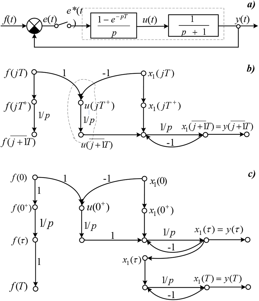
As an example in the Figure 4b has been demonstrated the simplex discrete system graph. Graph edge, match with fixing device, has been marked by dotted line. In the Figure 4c presented the graph for the case, when the mentioning occur within the interval τ = γT. As illustrated, in this case the graphs within the intervals $j T ÷ j + 1 ¯ T$ are presented as two split sub-graphs, one of which replies to fixing area, the other one – to signal capture failure area.

Fig. 4. The simplex discrete system and its SVG

Download Original Figure

Based on constructed SVG one may easily obtain recursions to solve analysis and synthesis matters.

3.2. Substandard Systems

Next consider state variables graphs for discrete systems with the pulse elements complex closure mode (of substandard systems). To substandard systems may be referred the systems with the switching cyclic frequency, with the pulse elements finishing closure time length, non-linear systems with the length-modulation.

Assume, that the switching basic time length within the system is equal to T. We divide this period into a number of various length intervals. This allow to determine easily the discrete system type and according to that to construct graph. Substandard system graph will contain a few sub-graphs, match with some intervals τ_i, which are the pieces of the basic period T.

To make a comparison, let’s consider first substandard discrete control systems calculation by state parameters space method [1]. For the interval

j T < t ≤ j T + t 1, (0 < t − j T ≤ t 1)

equation solution (1) will take the form

V → (t) = Φ → 0 (t − j T) ⋅ B → 0 ⋅ V → (j T)

(14)

o r V → (t) = H → 0 (t − j T) ⋅ V → (j T) .

(15)

Here $Φ → 0$ transfer matrix for this interval, and the transfer initial conditions shall be defined according to transient state formula

V → (j T +) = B → 0 ⋅ V → (j T) .

(16)

For the interval t₁ + jT < t ≤ jT + t₂, (t₁ < t − jT ≤ t₂) equation solution (1) will take a form:

V → (t) = Φ → 1 (t − j T − t 1) ⋅ B → 1 ⋅ V → (j T + t 1) = = H → 1 (t − j T − t 1) ⋅ V → (j T + t 1)

(17)

V → (t) = Φ → 1 (t − j T − t 1) ⋅ B → 1 ⋅ Φ → 0 (t 1) ⋅ B → 0 ⋅ V → (j T) = = H → 1 (t − j T − t 1) ⋅ H → 0 (t 1) ⋅ V → (j T) .

(18)

For interval t_i + jT < t ≤ jT + t_i+1, (t_i < t − jT ≤ t_i+1) equation solution (1) will write down in the form:

V → (t) = Φ → i (t − j T − t i) ⋅ B → i ⋅ V → (j T + t i)

(19)

V → (t) = Φ → i (t − j T − t i) ⋅ B → i ⋅ Φ → i − 1 (t i − t i − 1) ⋅ B → i − 1 ⋅ ... ... Φ → 1 (t 2 − t 1) ⋅ B → 1 ⋅ Φ → 0 (t 1) B → 0 ⋅ V → (j T) = = H → i (t − j T − t i) ⋅ H → i − 1 (t i − t i − 1) ⋅ ... ... H → 1 (t 2 − t 1) ⋅ H → 0 (t 1) ⋅ V → (j T) .

(20)

With respect to formulas (19), (20) the matrices $Φ → i, B → i, ⋅ H ¯ i$ could be different for different intervals of elementary switch period.

Thus, the state variables graph for substandard discrete systems it’s necessary to construct in several steps according to minor intervals number τ_i, i.e. the graph will consist of few sub-graphs, match with the intervals, $(j T < t ≤ j T + t 1), (j T + t 1 < t ≤ j T + t 2), …, (j T + t i < t ≤ j T + t i + 1), …, (j T + t k < t ≤ j + 1 ¯ T)$ .

It stands to reason, the structure and emissions valuations some sub-graphs in general case will be differed from one another. Each sub-graph will be built according to the system operation mode in terms of interval concerned τ_i. Sub-graphs jointing shall be performed given, that the state variables $V → (j T + t i)$ , calculated for the situation t_i = (t − jT), will come as sources-nodes for the next switch for interval (jT + t_i < t ≤ jT + t_i+1).

As an illustration in the Figures 5a, 5c presented repeated on-off signals system and its graph. Here the governor represented as pulsed filter in feedback circuit Switch periods T₁ = 1/2c and T₂ = 1/3c (Figure 5b), unit step function input signal, the initial conditions are supposed to be null.

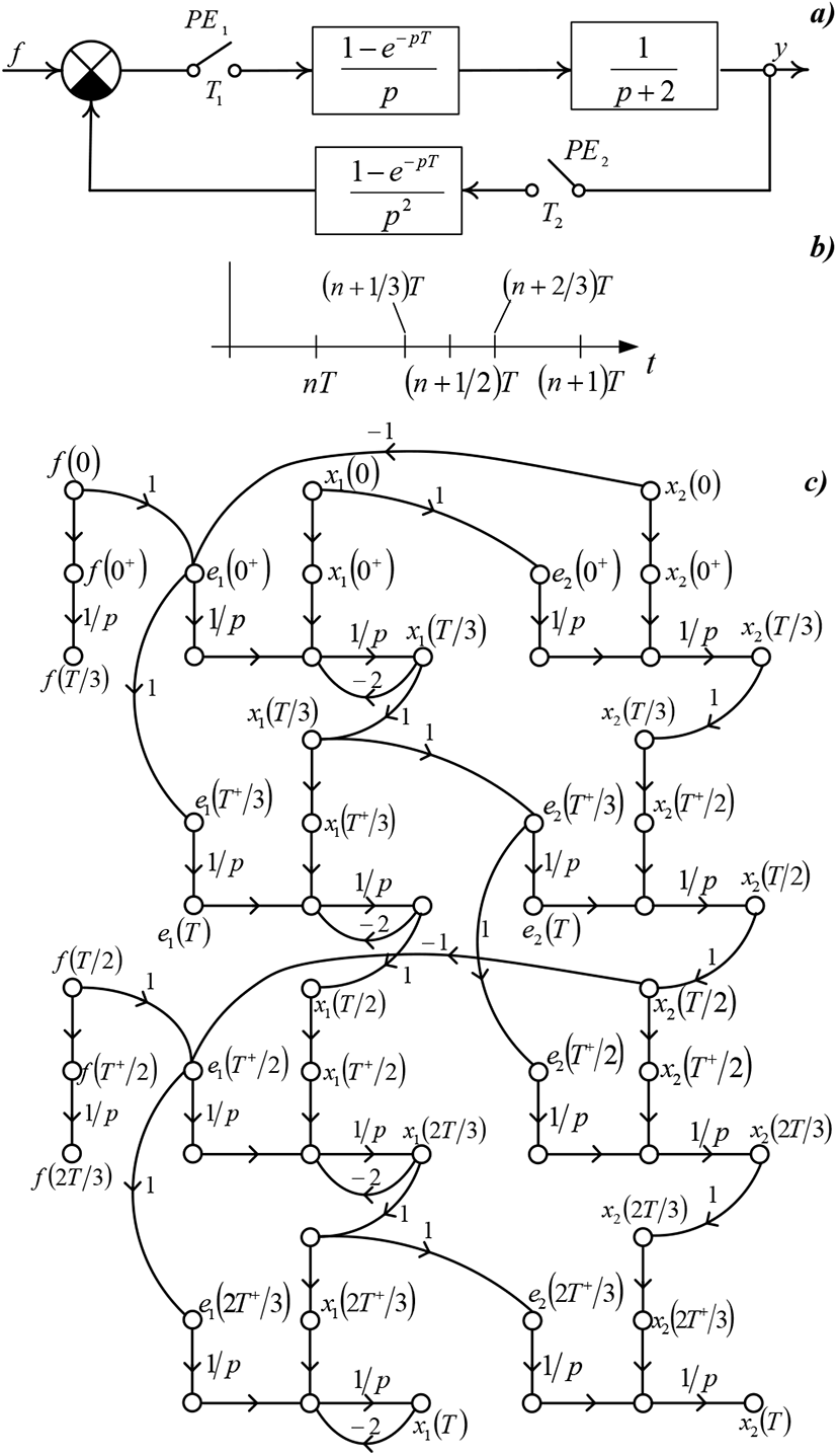
Fig. 5. Structural diagram and SVG of discrete system with repeated on-off signals

Download Original Figure

The complex discrete system state variables graph allows to describe, without gaps, the system status all over intervals of one period.

3.3. Multivariable Nonlinear Discrete Systems

Linearity separable within the nonlinear discrete systems graph models are presented as weighted emissions edges, that vary from time step to time step according to the law $e ⌢ i (j T) = Φ [e i (j T)]$ .

Or linearity may be presented as the enhancer with the variable gain constant k_j. The value k_j(j ∊ J = {0,1,…}) depends on nonlinear element characteristics and remains steady within the pulse element switch period.

State variables graph N -dimensional discrete system constructs in similar to previous cases, but will be appeared as combination of N² sub-graphs, match with transmissions channels, where N – present as constitution models of status N of separate transmission channels, and the rest (N² – N) indicate the switch-back transmission channels.

Let’s consider the multivariable nonlinear discrete systems SVG construction task based on separate elements models. Let’s introduce the signs, accessible in terms of multidimensional systems dynamics description: $F → r$ – input signal vector r-shape channel; $Y → r$ – output signal vector r-shape channel; $A → r$ – transition matrix (weighted transposed incident matrix) r-shape transmission channel; $C → r k$ – transition matrix (rk) switch-back channel (weighted transposed incident matrix). With scalar values $f n r, y n r, a j i r, c j i r k$ are marked accordingly the column-vectors components and state variables graph edges transmission factors.

To describe the multidimensional system transmission channels state variables let’s introduce the signs: $X ¯ r, X r$ – column-vector and state variables variety r-shape separate transmission channel; $X ¯ r k, X r k$ – column-vector and variety of state variables rk-shape switch-back transmission channel; $x l r – l$ state variable r-shape separate transmission channel; $x l r k – l$ state variable rk-shape switch-back transmission channel.

Top points $x i r (j + 1 ¯ T), x i r k (j + 1 ¯ T)$ present as the output vector components, the top points $x i r (j T), x r r k (j T), i = 1, 2, ..., n −$ input vector components of transmission channel, preset by its transition matrix

X → r (j + 1 T ¯) = A → r X → r (j T),

(21)

X → r k (j + 1 T ¯) = C → r k X → r k (j T) .

(22)

The signals within some spots shall be defined according to formulas:

x l r (j + 1 T ¯) = ∑ i = 1 n a l i r x i r (j T),

(23)

x l r k (j + 1 T ¯) = ∑ i = 1 n c l i r k x i r k (j T) .

(24)

Thus, the output signals r coordinate of N-dimensional of non-linear discrete system shall be defined out of the formula:

y r (j + 1 ¯ T) = x 1 r (j + 1 ¯ T) + ∑ k = 1, (k ≠ r) N x 1 r k (j + 1 ¯ T) .

(25)

Multidimensional control object graph model will result from the all separate and switch-back transmission channels models association:

G t = G t r U G t r k,

(26)

where

G t r = (X r (j T), X r (j + 1 ¯ T), V r) X r (j T) = (x i r (j T)); X i r (j + 1 ¯ T) = (x i r (j + 1 ¯ T)); V r = {〈 (x l r (j T), x m r (j + 1 ¯ T)), a m, l r (T)};

(27)

G t r k = (X r k (j T), X r k (j + 1 ¯ T), V r k) X r k (j T) = (x i r k (j T)); X r k (j + 1 ¯ T) = (x i r k (j + 1 ¯ T)); V r k = {〈 (x l r k (j T), x m r k (j + 1 ¯ T)), c m, l r k (T) 〉}; i, l, m = 1, 2, ..., n; r, k = 1, 2, ..., N; r ≠ k .

(28)

With regard to all stated let’s formulate the graph model construction algorithm for nonlinear multidimensional discrete systems:

Laid down the one time reference scale for pulse elements closure moments PE₁, PE₂,…, PE_N, :

$t ˜ * = t 1 ∪ t 2 ∪ ⋅ ⋅ ⋅ ∪ t N,$

wheretⁱ=(.), i=1, 2,…, N – the variety of closure momentsi pulse element.
Shall be constructed the input signals graph models (similar to continuous part models), forming units, pulse-wise components, nonlinear elements.
The entire system topological model constructs from the topological models separate parts with the provision for system microstructure and its observation interval across the axis $t ˜ *$ . If the system elements graph models been defined as $G t f = (f i, e i, V f)$ – input signals models, $G t N E = (e i, e^i, V N E) −$ nonlinear elements models, $G t P E = (e^i, e^i *, V P E) −$ pulse elements models, $G t = G t r ∪ G t r k$ – system continuous parts models, then the multidimensional nonlinear discrete system general graph model will be defined as the all these graph models association

G t c = G t f ∪ G t N E ∪ G t P E ∪ G t L F ∪ G t .

(29)

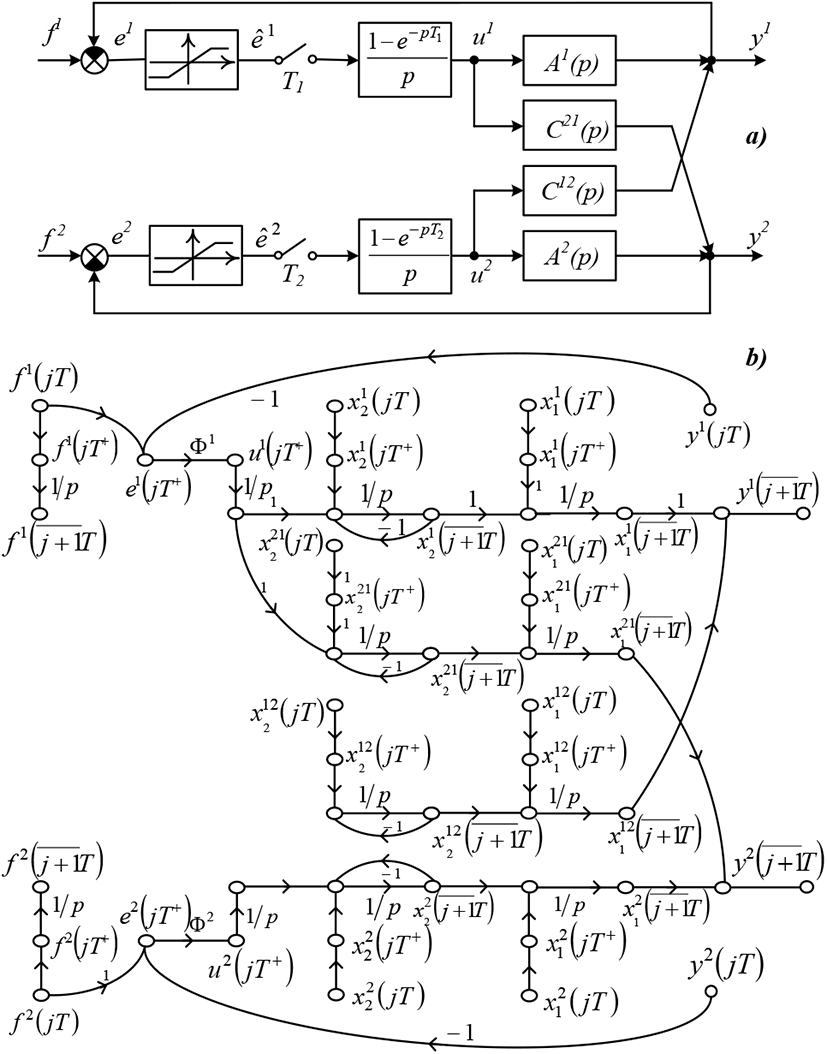
As an illustration in the Figures 6a, 6b demonstrated the bivariate structural diagram and the state variables graph match with.

Fig. 6. Non-linear discrete system (a), graph system model (b)

Download Original Figure

IV. DISCRETE SYSTEMS SYNTHESIS

Let’s consider the discrete system of n–order with the nonzero initial conditions. Task: to find the optimal controls subsequence and state feedback law, switching the control object from preset initial state $x → (0) ≠ 0 →$ to balance condition within the minimum time.

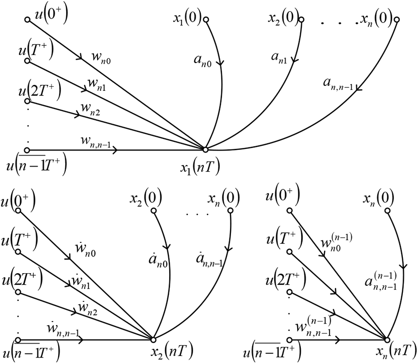
Let’s assume that the balanced state is the state, when the all system coordinates take up the zero value, i.e. $x → (l T) ≠ 0 →$ where l = n for controls free systems and l = n + g – if actuating signals restrictions. Prior to switch to HGM presented of continuous system part, need to decide the state variables and construct the state variables graph. Based on graph one may find weighting function and its derivatives $a (t), a ˙ (t), ..., a (n − 1) (t)$ of the object itself and weighting function and its derivatives of presented continuous part $w (t), w ˙ (t), ..., w (n − 1) (t)$ . Making coefficients sample capture, weighting functions were obtained with T interval (T – is the signals sampling time object input), do construction HGM for the interval (0; nT). The latter represents as n sub-graphs, constructed for each system coordinate separately (Figure 7).

Fig. 7. The system HGM

Download Original Figure

Straight by sub-graphs sight one may write the process state equation for balance point:

x 1 (n T) = a n 0 x 1 (0) + a n 1 x 2 (0) + ... + a n, n − 1 x n (0) + + w n 0 u (0 +) + w n 1 u (T +) + ... + w n, n − 1 u (n − 1 ¯ T +); x 2 (n T) = a ˙ n 2 x 2 (0) + a ˙ n 3 x 3 (0) + ... + a ˙ n, n − 1 x n (0) + + w ˙ n 0 u (0 +) + w ˙ n 1 u (T +) + ... + w ˙ n, n − 1 u (n − 1 ¯ T +); ..................................................................... x n (n T) = a n, n − 1 (n − 1) x n (0) + w n 0 (n − 1) u (0 +) + + w n 1 (n − 1) u (T +) + ... + w n, n − 1 (n − 1) u (n − 1 ¯ T +) .

(30)

If we substitute to (30) the highest response speed conditions x₁(nT = 0;x₂(nT = 0;…; x_n(nT = 0;, will obtain the equations required best sequence ${u (j T +)} = {u (0 +), {u (T +), ..., {u (n − 1 ¯ T +)}$ for case, when no restrictions for equations.

To discover the optimal control law it is required to define the control action u(jT⁺) as state coordinate function

u (j T +) = β 1 x 1 (j T) + β 2 x 2 (j T) + ... + β n x n (j T) .

(31)

The feedback coefficients may be discovered according to the same hybrid graph model. Let’s substitute the obtained control values in formulas (30) type and will define state coordinates values in instants earlier, i.e. the values

x 1 (T), x 2 (T), ..., x n (T); x 1 (2 T), x 2 (2 T), ..., x n (2 T); ...; x 1 (n − 1 ¯ T), x 2 (n − 1 ¯ T), ..., x n (n − 1 ¯ T) .

Finally will obtain the following the non-homogeneous equations linear system:

u (0 +) = β 1 x 1 (0) + β 2 x 2 (0) + ... + β n x n (0) u (T +) = β 1 x 1 (T) + β 2 x 2 (T) + ... + β n x n (T) ................................................................ u (n − 1 ¯ T) = β 1 x 1 (n − 1 ¯ T) + β 2 x 2 (n − 1 ¯ T) + ... + β n x n (n − 1 ¯ T)}

(32)

Based on that will find the desired feedback coefficients, being the inverse matrix elements according to:

β → = [β 1 β 2 ... β n]

(33)

In the event of pulse elements complex operating mode discrete system, computing chain will be unchanged. It’s just enough to make the required sample capture of weighting function coefficients as well as its derivatives with provision for sampling moments. If there have been applied restrictions for actuating signals saturation type, the response time will be going up, that is why the hybrid graph need to be constructed for interval as $(0, n + g ¯ T)$ .

Based on mentioned above, we will formulate the optimum controls computation chain algorithm and inverse matrix of system discrete with the initial potential energy:

Based on system continuous part transfer function do construction of SVG and find the weighting functions a(t) object, presented continuous part of w(t) and its derivatives $a ˙ (t), ..., a (n − 1) (t); w ˙ (t), ..., w (n − 1) (t)$ .
Based on the pulse elements operating mode we do make weighting functions coefficients sample capture, $a j i, a ˙ j i, ..., a j i (n − 1); w j i, w ˙ j i, ..., w j i (n − 1)$ , j – epoch of observation, i – epoch of pulse advent (j=0, 1,…, n+g; i=0, 1,…, n+g).
Do construction the hybrid graph model for the moment t=nT, based on that, will find the state variables $x → (n T)$ towards the initial state function $x → (0)$ and controls sequence {u(jT⁺)}, j = 0,1,…,n − 1..
Considering, that $x → (n T) = 0 →$ , will define out of obtained in point 3 equation the sequence {u(jT⁺)},. If the all controls are located within the limiting levels, will switch to point 6, otherwise will implement point 5.
Will do increase the hybrid graph size by one step and again will find the controls {u(jT⁺)}, j = 0,1,…,n. Will continue the process, until the all controls will be located within the required extents.
Based on hybrid graph we do define the system state variables values in terms of sampling moments $t = T, 2 T, ..., n + g − 1 ¯ T$ .
Expressing each control signal u(jT⁺) through the state coordinates values x₁(jT), x₂(jT),…,x_n(jT), we do compose set of equations (32), based on that solution will find the inverse matrix elements $β →$ .
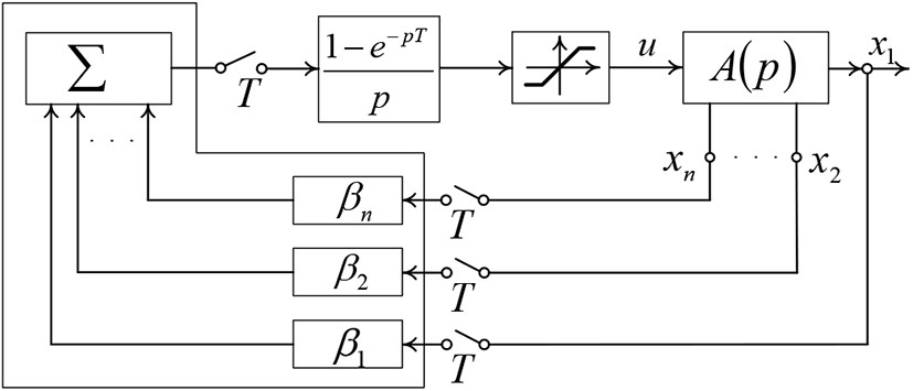
Let’s construct the synthesized system diagram (Figure 8).

Fig. 8. Synthesized digital system diagram

Download Original Figure

V. GRAPHICAL EXAMPLE

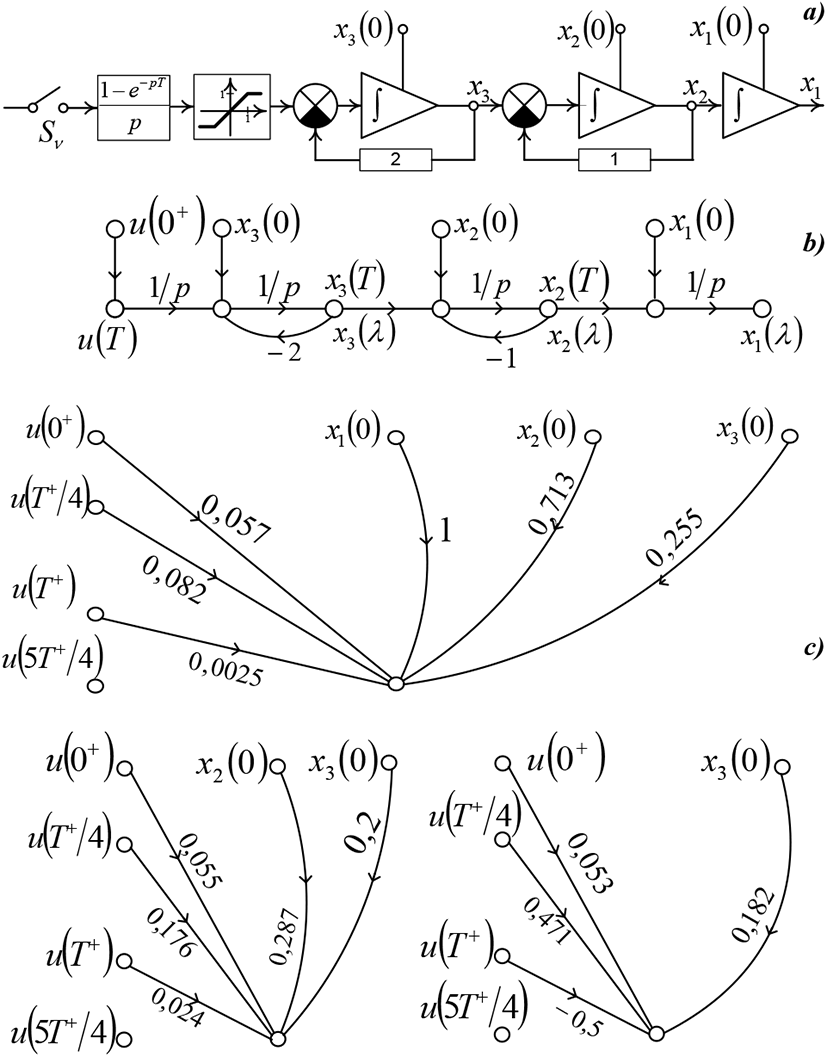
In Figure 9a was demonstrated the input signal cycle frequency of interruption system diagram. Such process is characterized by transfer function as below

A (p) = 1 p (p + 1) (p + 2) .

Fig. 9. State variables diagram, SVG and HGM systems

Download Original Figure

The interrupter S_v makes sample capture from the signal at the instants of time t = 0,T/4,T,…jT, (j + 1/4)T,…. Switching time T=1c, initial state vector $x → (0) = [0, 10, 10, 1] ′$ . There has been imposed restrictions to control actions |u| ≤ 1. It is required to find the minimum number of steps, that are required for process relocation from preset initial state to balanced conditions, and define the optimal control sequence {u(jT⁺)}, and optimum control law.

The computing chain as follows.

Do construction of state variables graph the presented continuous part (Figure 9b). Based on that will find the weighting functions and its derivatives:

$w (t) = 0, 25 (2 t − 3 + 4 e − t − e − 2 t); w ¨ (t) = 0, 5 (1 − e − 2 t); w ˙ (t) = 0, 5 (1 − 2 e − t + e − 2 t); a 1 (t) = 1; a 2 (t) = 1 − e − t; a 3 (t) = 0, 5 (1 − 2 e − t + e − 2 t); a ˙ 1 (t) = 0; a ˙ 2 (t) = e − t; a ˙ 3 (t) = e − t − e − 2 t; a ¨ 1 (t) = 0; a ¨ 2 (t) = 0; a ¨ 3 (t) = e − 2 t .$

$w (t) = 0, 25 (2 t − 3 + 4 e − t − e − 2 t); w ¨ (t) = 0, 5 (1 − e − 2 t); w ˙ (t) = 0, 5 (1 − 2 e − t + e − 2 t); a 1 (t) = 1; a 2 (t) = 1 − e − t; a 3 (t) = 0, 5 (1 − 2 e − t + e − 2 t); a ˙ 1 (t) = 0; a ˙ 2 (t) = e − t; a ˙ 3 (t) = e − t − e − 2 t; a ¨ 1 (t) = 0; a ¨ 2 (t) = 0; a ¨ 3 (t) = e − 2 t .$
Considering pulse elements operating mode will do sample capture of weighting functions coefficients.
Do construction of hybrid graph model as three un-jointed sub-graphs for the moment t=5T/4 (Figures 9c, 9d). Will find the state variables

$x 1 (5 T / 4) = x 1 (0) + 0, 713 x 2 (0) + 0, 255 x 3 (0) + 0, 057 u (0 +) + 0, 082 u (T + / 4) + 0, 0025 u (T +); x 2 (5 T / 4) = 0, 287 x 2 (0) + 0, 2 x 3 (0) + 0, 055 u (0 +) + 0, 176 u (T + / 4) + 0, 024 u (T +); x 3 (5 T / 4) = 0, 182 x 3 (0) + 0, 053 u (0 +) + 0, 0471 u (T + / 4) + (− 0, 5) u (T +) .$
The minimum number of steps in linear system shall be defined by object degree of a differential equation. For system concerned it’s equal three.

$x 1 (5 T / 4) = x 2 (5 T / 4) = x 3 (5 T / 4) = 0.$

Based on obtained in point 3 equations will define the sequence {u(jT⁺)}

${u (j T +)} = {− 5, 45; 1, 328; 0, 71} .$
Since the equation u(0⁺) exeeds the limiting level |u_max>| = 1, we switch to next step.

We compose the equations for the moment t=2T. Constitutive equations for this instant considering the maximum response speed terms $x → (2 T) = 0 →$ and initial conditions appear as:

$0, 088 u (0 +) + 0, 207 u (T 4 +) + 0, 04 u (T +) + 0, 041 u (5 T 4 +) = − 0, 133 0, 033 u (0 +) + 0, 141 u (T 4 +) + 0, 06 u (T +) + 0, 14 u (5 T 4 +) = 0, 0078 0, 012 u (0 +) + 0, 105 u (T 4 +) + 0, 088 u (T +) + 0, 777 u (5 T 4 +) = 0, 0102}$

Based on that will find the following controls sequence:

${u (j T +)} = {− 1; − 1, 45; 4, 139; − 0, 26} .$

Being that again in this sequence is the control, exceeding the limiting level, We increase the transient time one step more. Will find the state variables x₁(9T/4); x₂(9T/4); x₃(9T/4);.

Assuming $x → (9 T / 4) = 0 →$ and considering, that $x → (0) = [0, 10, 10, 1] ′$ , will obtain

${u (j T +)} = {− 1; − 0, 692; 1; 0, 2273; − 0, 279} .$

Controls computation thereon could be completed, since the all controls at sequence {u(jT⁺)} are within the limiting level, and consider, that process from initial state $x → (0)$ to balanced state could be transferred within the minimum number of steps equal 5.
According to weighting functions and equations found {u(jT⁺)};j = 0, 1/4, 1, 5/4, 2 will find the state coordinates values at sampling moments.

Express the controls {u(jT⁺)};j = 1/4, 5/4, 2 through the state variables values x₁(jT), x₂(jT), x₃(jT), will obtain the equations system:

$u (T 4 +) = β 1 x 1 (T 4) + β 2 x 2 (T 4) + β 3 x 3 (T 4) u (5 T 4 +) = β 1 x 1 (5 T 4) + β 2 x 2 (5 T 4) + β 3 x 3 (5 T 4) u (2 T +) = β 1 x 1 (2 T) + β 2 x 2 (2 T) + β 3 x 3 (2 T)},$
Substitute the controls values and state variables, will find the inverse matrix elements:

$B → = {− 5, 778; − 2, 397; − 4, 97} .$
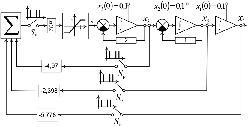
Do construct the synthesized digital system diagram (Figure 10).

Fig. 10. Synthesized system diagram

Download Original Figure

VI. CONCLUSION

Thus, we demonstrated, how with the aid of dynamic graph models could be constructed the diverse discrete systems models. Suggested graph models allow to cover such systems classes, like nonlinear with pulse-duration modulation, systems with the cycling interruption rate, with the finite quantization time, nonlinear continuous parts systems, linear and nonlinear multidimensional systems. Such give a chance to obtain an attractive in terms of calculating, formulas to calculate transients for all under the measurement coordinates; to do research of all mentioned classes and systems in terms of stability; to determine its controlled and observable coordinates.

The developed models and algorithms significantly simplify the analysis and synthesis complex discrete systems tasks solution, since according to graph models there is a chance to write out the equations required at one, with no extra operations, are associated in state variables method with the necessity for repeated multiplying out and matrixes inversion.

REFERENCES

[1].

Tu Yu, Current Control Theory. Transl. from eng. Under the editorship V.V.Solodovnikov. Moscow: Engineering, 1971.

[2].

L. T. Kuzin, Calculation and Design of Discrete Control Systems. Moscow: Mashgiz, 1962.

[3].

S. Mezon and Zimmerman, Electronic Circuits, Signals and Systems. Transl. from eng. Moscow: Foreign literature, 1963.

[4].

A. A. Kadirov, Dynamic Graph Models in Control Systems. Tashkent: Fun, 1984.

[5].

V. N. Fomin, Methods of Control by Linear Discrete Objects. Leningrad: LSU, 1985.

[6].

L. N. Volgin, The optimal discrete control by dynamic systems. -M.: Science, 1986.

[7].

V.M. Matrosov, S.N. Vasiliev and A.I. Moskalenko, Nonlinear control theory: dynamics, control, optimization. Under the editorship. Moscow: Physmatlit, 2003.

[8].

Ling Hou and Anthony N. Michel, “Unifying theory for stability of continuous, discontinuous, and discrete-time dynamical systems,” Nonlinear Analysis: Hybrid Systems, vol. 1, no. 2, pp. 154-172, 2007.

[9].

Rafal Goebel, G. Ricardo. Sanfelice and Andrew R. Teel, Hybrid Dynamical Systems. PrincetonUniversity Press, 2012. 227 p.

[10].

D. Mignone, “Control and Estimation of Hybrid Systems with Mathematical Optimization,” A dissertation submitted to the Swiss Federal Institute of Technology (ETH), Zurich for the degree of Dr. sc. techn., 2002.

[11].

A.A. Kadirova, The Modeling Methods and Research of Nonlinear and Logical-Dynamic Control Systems. Tashkent: Yangi Asr Avlodi, 2010.