I. INTRODUCTION
The strong nonlinear behavior and uncertainties of many practical systems and the unavailability of quantitative data regarding the input-output relations make an analytic approach to the behavior analysis of the system even more difficult. Hence, many engineers and scientists have focused their attentions on the computational intelligence-based approaches such as fuzzy logic, neural network, genetic algorithms and etc. In spite of many practical successes, the process for fine tuning of fuzzy control rules in order to get the desired performance is a time-consuming and tedious task even though linguistic control rules are extracted from experts’ knowledge. To overcome these difficulties, the self-organizing fuzzy controller was proposed by Mamdani[1] and extended by others.
The simulated annealing technique was introduced by Kirkpatrick et. al.[2] in 1983. The foundations for this algorithm are given by Matropolis et. al. [3]. The simulated annealing algorithm is based on an analogy with the annealing of solids. Downhill moves are always accepted, whereas uphill moves are accepted with the probability that is a function of temperature.
Random signal-based learning [4], introduced by authors of this paper, is similar to a reinforcement learning of neural network using random signal. The learning object is learned by the value which is generated through the activation function (bipolar step function), which input is random signal, and then compare the performance index with the prior step to generate the reinforcement signal.
This paper describes the application of simulated annealing to a random signal-based learning. The simulated annealing is used to generate the reinforcement signal which is used in the random signal-based learning. Random signal-based learning is poor at hill-climbing, whereas the simulated annealing has an ability of probabilistic hill-climbing. Therefore, hybridizing a random signal-based learning with simulated annealing can produce better performance than before. The validity of the proposed algorithm is confirmed by applying it to two different examples. One is finding the minimum of the nonlinear function. And the other is the optimization of fuzzy control rules using inverted pendulum. The key of this example is to adjust both the width and the center of membership functions so that the tuned rule-based fuzzy controller can generate the desired performance.
II. RANDOM SIGNAL-BASED LEARNING
The learning of neural networks is the process which its synapse strength is changed according to the prescribed rules to store any information in it. Hebb [5] presented the learning rules as follows: When two neurons A and B are interconnected with each other, if the neuron A is activated, the other neuron B is also activated. As a result, the synapse strength between A and B is represented as
where m is the synapse strength, η is a learning coefficient and y is the output of a system. By the way, synaptic equilibrium occurs in steady state when the synaptic strength m stops moving, that is,
For intentional learning, we intentionally add Gaussian white noise process n(t) to eq. (2). Then the synaptic strength m reaches stochastic equilibrium when only the random noise vector n changes m, that is, ṁ(t) = n(t). Then, the zero means noise property of eq. (2) and the stochastic equilibrium condition ṁ(t) = n(t) implies the average equilibrium condition
reaches equilibrium.
The learning law takes the following form:
where η : learning rate
f : activation function
n : discrete random process with values between 0 and 1
θ : bias (=0.5)
r(t) : reinforcement signal
and the reinforcement signal r(t) is defined as follows:
where
In this learning law, synapses learn when only a performance index is decreased after the learning. In other words, r(t) of eq. (4) will be set by 1. Otherwise, the learning will be rejected, that is, r(t) of eq. (4) will be set by 0. The activation function f is a bipolar sigmoid function as following form:
III. SIMULATED ANNEALING
The simulated annealing is a method that has attracted significant attention for large-scale optimization problems that have many local minima and make reaching the global minimum difficulty.
The idea of the simulated annealing comes from the physical annealing process done on metals and other substances. In metallurgical annealing, a metal body is heated to near its melting point and then slowly cooled back down to room temperature. This process will cause the global energy function of the metal to reach on the absolute minimum value eventually. If the temperature is dropped too quickly, the energy of the metallic lattice will be much higher than this minimum because of the existence of frozen lattice dislocations that would otherwise eventually disappear because of thermal agitation.
Analogous to this physical behavior, the simulated annealing allows a system to change its state to a higher energy state occasionally such that it has a chance to jump out of the local minima and seek the global minimum. The function to be minimized i.e., the performance index, is analogous to the energy of metal, and the control parameter, called temperature, is analogous to the temperature of metal. Downhill moves are always accepted, whereas uphill moves are accepted with the probability that is a function of temperature. The acceptance probability is usually given by the Boltzmann distribution,
where ΔE is the change in the performance index and T is the temperature. If ΔE is negative then the new solution is always accepted. If ΔE is positive then the new solution could be accepted with the probability in eq. (7). The possibility of accepting the uphill movement permits escaping from the local minima.
After the decision of acceptance of a new solution, the temperature is adjusted by cooling schedule, and the process is repeated until some convergence conditions are reached. Because of its speed, exponential cooling schedule is used in this research. The temperature at any stage during the optimization may be expressed as follows:
where T0 is initial temperature that is large enough, α is cooling rate and k is time index.
IV. PROPOSED ALGORITHM
In this paper, we propose the application of simulated annealing to a random signal-based learning, that is, we use the simulated annealing to generate the reinforcement signal r(t) in eq. (4). In eq. (7), ΔE is defined as follows:
where J(t) is performance index.
In eq. (9), if ΔE is negative then the new solution is always accepted. If ΔE is positive then the new solution could be accepted when only the acceptance probability p in eq.(7) is greater than the random number between 0 and 1.
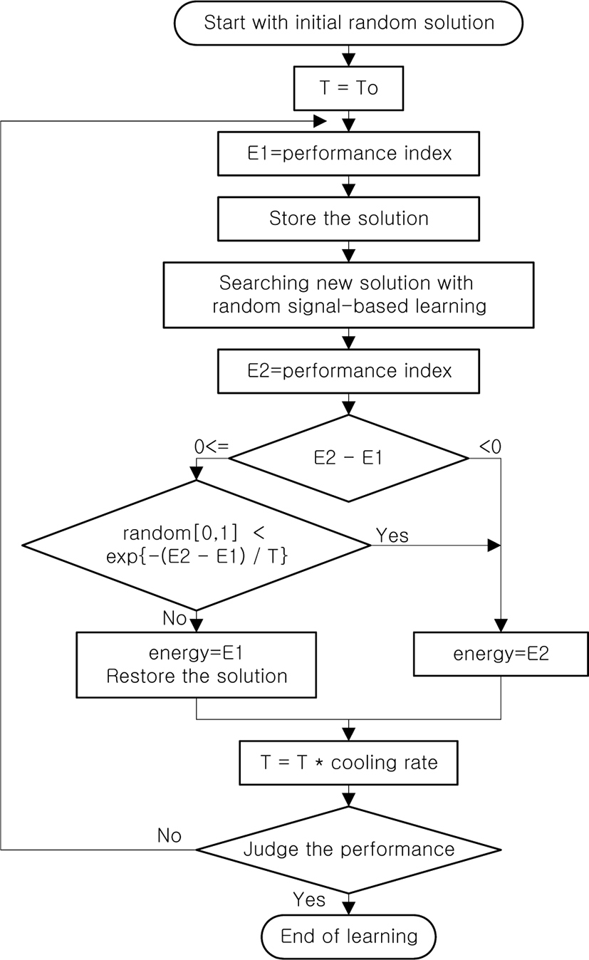
Figure 1 shows the proposed algorithm. The proposed algorithm can be described as follows:
-
Step 1. Start with initial random solution: Initial solution is chosen at random.
-
Step 2. T=To: Put initial temperature To into temperature, T.
-
Step 3. E1=performance index: Put the performance index, which is evaluated using current solution, into E1.
-
Step 4. Store the solution: Store the current solution in arbitrary memory location.
-
Step 5. Searching new solution with random signal-based learning: The solution is learned by random signal-based learning.
-
Step 6. E2=performance index: Put the performance index, which is evaluated using new solution, into E2.
-
Step 7. E2-E1: If E2 is less than E1 then put E2 into energy and goto Step 9. Else goto next Step.
-
Step 8. random[0,1]<exp[-(E2-E1)/T]: If the acceptance probability is greater than random number between 0 and 1 then put E2 into energy. Else put E1 into energy and restore the solution before learning in Step 4.
-
Step 9. T=T*cooling rate: Multiply T by cooling rate.
-
Step 10. Judge the performance: If the stopping criterion is satisfied then end algorithm. Else goto Step 3 and repeat until the stopping criterion is satisfied.
V. SIMULATION RESULTS
The validity of the proposed algorithm is confirmed by applying it to two different examples.
One is finding the minimum of the nonlinear function F(x) in eq. (10)[6].
where −1<x<1.
Initial temperature T0 is 200, α is 0.98, learning rate η is 0.01 and the performance index of this example is F(x) itself because the purpose is to find x which minimize F(x).
Figure 2 shows x and nonlinear function F(x). F(x) has two local minima as well as the global minimum in the specified region of x. We know by calculation that the true solution is about 0.07715.
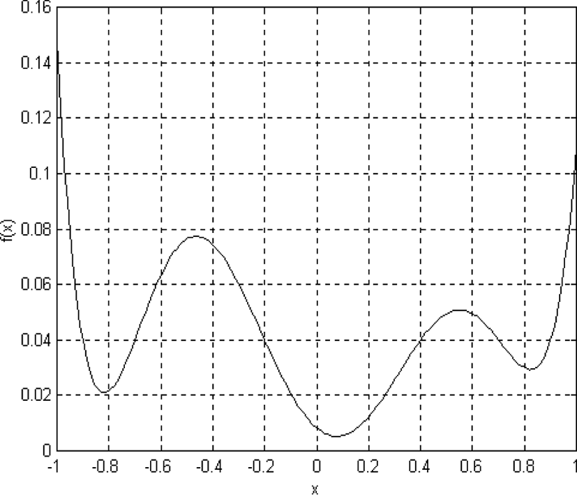
Figure 2 shows x and nonlinear function F(x). F(x) has two local minima as well as the global minimum in the specified region of x. We know by calculation that the true solution is about 0.07715.
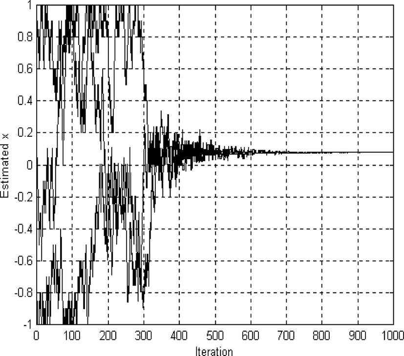
Figure 3 shows the estimated x in each iteration for different initial conditions (-0.8, 0.1, 0.9) and eventually converge on the global minimum (x=0.0771).
Another example is control of the inverted pendulum using a fuzzy controller. A mathematical model of the inverted pendulum system can be derived as follows:
where mass of cart M is 3Kg, length of pole l is 0.6m and mass of pole m is 0.1Kg. Initial temperature T0 is 0.05, α is 0.98, learning rate η is 0.01 and the performance index of this example is like this:
where e is error, ė is derivative of error and k is the number of input-output pair. The performance index is evaluated by control of the inverted pendulum in constant time.
The number of linguistic variable is 5 and we control only angle of the inverted pendulum. Antecedent parts are fixed and only consequent parts of the fuzzy control rules are considered to learn for our simplicity. That is, the key of this example is to adjust both the width and the center of consequent part membership functions so that the tuned rule-based fuzzy controller can generate the desired performance. The number of centers and widths are 25 respectively because the number of linguistic variable is 5.
To show the effectiveness of the proposed algorithms, the simulations of genetic algorithms and the random signal-based learning are achieved respectively. In genetic algorithms, population size is 10, maximum generation is 100, crossover probability is 0.6, mutation probability is 0.013 and all conditions are the same as the proposed algorithm. Also, the parameters and conditions of the random signal-based learning are the same as the proposed algorithm.
Figure 4 shows the structure of self-learning fuzzy controller using the proposed algorithm.
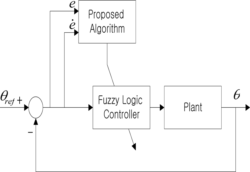
Table 1, table 2, and table 3 show final centers and widths learned by the proposed algorithm, the random signal-based learning and the genetic algorithms respectively.
Figure 5 shows the controlled output of the inverted pendulum obtained by using the fuzzy control rules after the learning, i.e., table 1, table2 and table 3. The control parameters are the same as during the learning. The proposed algorithm and the random signal-based learning are learned until the performance index is not changed. The genetic algorithm is learned during 100 generations. The variation around 10sec is disturbance. The result shows that the control performance of the proposed algorithm is greatly enhanced in convergence time and the disturbance than the genetic algorithm and the random signal-based learning. Especially, comparing the computational time of the proposed algorithm with that of the genetic algorithms, the proposed algorithm is shorter than the genetic algorithms.
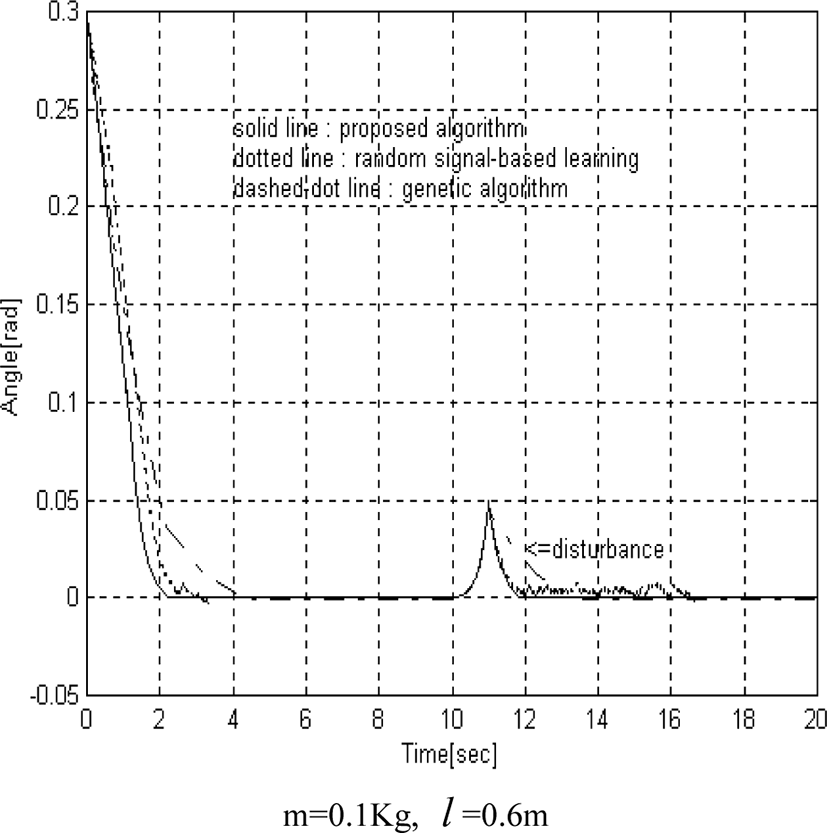
Figure 6 shows the controlled output of the inverted pendulum obtained by using the fuzzy control rules after the learning. In this case, the control parameters are different from the learning, that is, m=0.2Kg, l =1.2m. And also, the variation around 10sec is disturbance. From the result, we can see that the proposed algorithm is more robust in parameter change than other both cases.
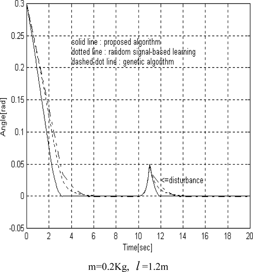
Figure 7 shows energy profile during the learning. In this figure, energy moves uphill and downhill according to the acceptance probability p in eq. (9) and finally reaches 0 energy state, i. e., to near the global minimum.
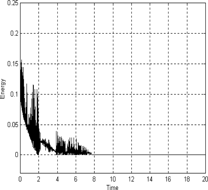
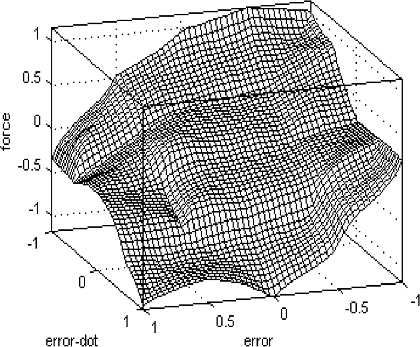
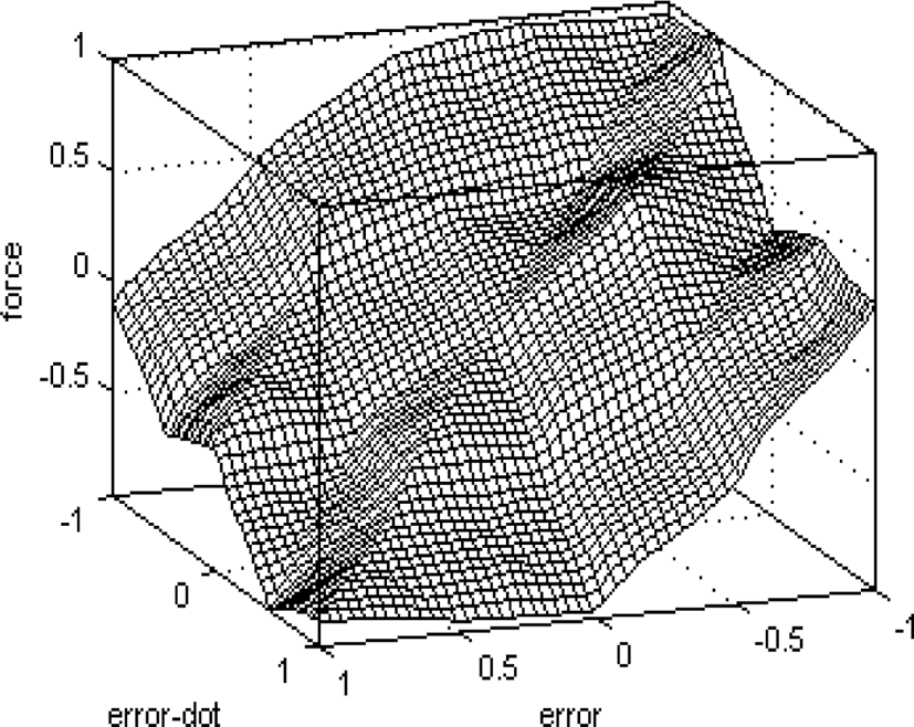
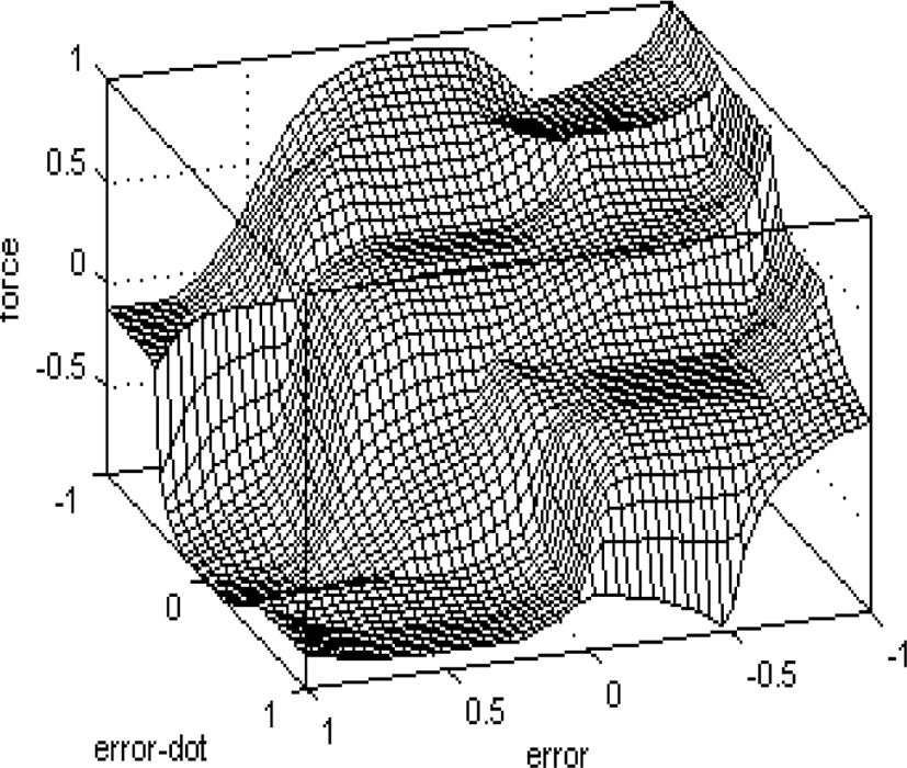
Fig. 8, Fig.9 and Fig. 10 show control input space of the proposed algorithm, the random signal-based learning and the genetic algorithm respectively. In Fig. 8, we expect that the settling time is very short because the gradient of surface around 0 varies smoothly. In Fig. 9, we expect that the chattering phenomenon occurs because it has sharp convex and concave. And in Fig. 10, we also expect that settling time is very long because it has the region that the gradient of surface does not vary.
VI. CONCLUSIONS
This paper was described the application of the simulated annealing to a random signal-based learning. The simulated annealing was used to generate the reinforcement signal which was used in the random signal-based learning. The validity of the proposed algorithm was confirmed by using two different examples. From the results, we expect that the proposed algorithm can be applied another optimization and control problems.