I. INTRODUCTION
In 1906, Alzheimer’s disease (AD) was first defined by Alois Alzheimer [1]. AD is a brain disease that is a major health problem in elderly humans. Death is inevitable in AD, and it is the sixth disease that causes most deaths around the world [3-4]. The estimated number of people with AD is about 30 million [3]. Destruction of neurons causes changes in the brain. Only after few years, the symptoms of AD are seen in patients [2]. The symptoms include changes in personality, poor judgment, abnormalities in mood, and sleep [2]. Identifying the transition in the progressive disorder of AD is challenging. AD patient’s diagnosis includes a collection of his/her history, neurological and laboratory examinations, and neuroimaging [1].
First, deposits of amyloid β-peptide (Aβ) appear to be neuropathological features of AD [5]. Amyloid precursor protein (APP) generates Aβ peptide. The activity of β-secretase and γ-secretase generates the Aβ peptide Aβ42, which is a longer species, initiates the deposition of amyloid [1]. Another feature of AD appears due to the accumulation of neurofibrillary tangles [5]. Tau protein is responsible for this phenomenon. Tangle formation is proportional to the severity of the disease. More tau tangles lead to severe conditions of AD [1]. Mild Cognitive Impairment (MCI) can be referred to as a phase of AD, in which the symptoms can be observed. Most commonly, the symptoms include a decrease in the ability to learn, unable to perform daily actions which were performed in past, require assistance for the daily activities [6].
For the analysis of the brain, the most used technique is Magnetic resonance imaging (MRI). MRI produces images in a non-invasive imaging technique. With the repetition of varied excitation, MRI produces an image of contrast in tissue for structures of interest [7]. There is a successive pulse sequence time interval, called Repetition Time (TR) and the time interval between delivery and reception of RF pulse and echo signal respectively is Time to Echo (TE). T1-weighted images generate common structural analytical annotation of tissues [8]. In T1-weighted images, both TR and TE times are short [8].
Information about the brain can be represented as an atlas. Desikan-Killiany-Tourville (DKT) atlas uses information based on curvature to define the regions of the brain. For defining the cortical regions in the DKT atlas, it is assumed that the curvature information on the inflated surface would help to gain high accuracy [9]. By using the mean distance of “mislabeling”, DKT atlas detects the geographical mismatch between regions [9]. By the study of brain atlas, the significant changes in the brain due to AD had been noticed [10]. For the analysis of the brain, atlas choice is very important. Researches have shown that the DKT atlas is able to identify significant differences between AD and CN group. In [10], 11 out of 62 structures were found to have a larger percentage difference between AD and CN.
The most commonly used workflow of studies includes feature extraction followed by classification. Many machine learning methods are available for classification. In [11], Support Vector Machine (SVM) classified four groups related to AD. Some studies [12, 13, 32, 25] classified groups using multiple classifiers. In these studies, the basic idea is to find the best classifier or to combine them for better results. Like in [13], classification using Softmax classifier, K-Nearest Neighbor (KNN), SVM, and Naive Bayes (NB) is compared for the best classifier. In [12], the combination of SVM, KNN, and Random Forest (RF) got higher accuracy than using them individually. SVM is found to be widely used in most cases. Modified SVM like Twin-SVM is also used in the classification [14].
Deep Neural Network (DNN) is the most common method which allows machines to perform multiple functions such as classification, analysis, and prediction [15]. Generally, a dense neural network also referred to as Fully Connected (FC) layer, consists of a large portion of the parameters of DNN [16]. In [17], the classification of AD is studied using an FC neural network. In most of the traditional AD analysis methods, many modalities are used at once to improve the performance of the system. Processing multiple modalities require an enormous amount of time followed by several feature selection methods. Only then some levels of satisfactory results were obtained. But these better results are not consistent among different datasets or different traditional classification models. In order to address these problems related with requirement of multiple numbers of modalities, classifiers and, feature extraction methods we propose a binary classifier based on a dense neural network. For this study, we used MRI images of only one modality (T1-weighted). The purpose of testing and comparing activation functions is to choose suitable activation functions that will help the model to learn even from the negative values.
In this study, we develop an FC neural network for the improvement in classification of AD with binary classification task. First, we processed the 3D images obtained from ADNI dataset using the FreeSurfer software. From FreeSurfer, we get atlas as features of the brain. The feature extraction process is followed by feature filtering using Principal Component Analysis (PCA) which allows feature selection, which is then followed by the classification. The proposed FC neural network comprises two hidden layers. Within those hidden layers, three different activation functions are tested for validation. A combination of activation functions from Parametric ReLU (PReLU), Leaky ReLU, and Exponential Linear Unit (ELU) is selected which has the highest validation accuracy. We performed 5-fold cross validation. After identifying, the model with the best validation accuracy, we used the ssame model to classify the test data for different group classification. This FC neural network performs as a binary classifier.
The contributions of this paper are summarized as follows:
-
We propose the combination of two out of three activation functions in the dense neural network with the best validation accuracy.
-
We propose use of combination of PCA with the dense neural network for the dimension reduction and feature selection to reduce manual task of filtering features.
-
We compare result of our model with the traditional machine learning methods on the same data and compared the result with the previous studies done with the same kind of data and processes.
Our contribution is to introduce a novel method of binary classification for AD detection with higher accuracy than other traditional methods. Furthermore, this system can be utilized in the early diagnosis of various stages of AD patients. Our aim is to develop a system that requires fewer resources but performs better than previous methods. The effectiveness of our proposed model is shown using accuracy, sensitivity, specificity, and bar plot for the comparison with traditional machine learning models.
The paper is arranged as follow: Section II consists of information about materials and methods along with the proposed classifier model; Section III conducts experiments using different activations functions and their results; Section IV shows the comparison of the proposed model with previous models and discussion; finally, the conclusion with the summarization of the paper is in Section V.
II. MATERIAL AND METHOD
In our study, we accessed data available on Alzheimer’s Disease Neuroimaging Initiative (ADNI). It was initiated with the primary objective to investigate whether imaging modalities can measure the progression or early detection of AD.
The dataset consists of 3 groups: AD, MCI, and Cognitively Normal (CN). Total of 178 subjects: 58 AD subjects (21 female, 37 male; age±SD = 75.3±7.9 years; education level = 15.1±3.4), 60 MCI (34 female, 26 male; age±SD = 74.5±3.8 years; education level = 15.2±2.5), and 60 CN subjects (27 female, 33 male; age±SD = 76.4±4.5 years; education level = 15.5±2.8) as shown in Table 1.
| Group | AD | MCI | CN |
|---|---|---|---|
| Nos. of subject | 58 | 60 | 60 |
| Female/male | 21/37 | 34/26 | 27/33 |
| Age | 75.3 7.9 | 74.5 3.8 | 76.4 4.5 |
| Education | 15.1 3.4 | 15.2 2.5 | 15.5 2.8 |
| CDR | 0.7 0.2 | 0.5 | 0 |
We used equal number of subjects in all groups, to have performance with unbiased estimations. The dataset is split into two parts, 80:20 ratio for training and for testing parts, respectively. The training data is further divided for the training and validation process. The model with the best validation accuracy score is then trained and finally, used to predict test data.
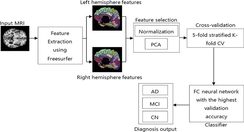
After data collection, we extracted features from those images in the next step. Fig. 1 shows the proposed method with the remaining processes. For this study, we ran FreeSurfer using the full recon-all pipeline to compute the DKT atlas which consists of cortical volumetric features. DKT atlas comprises 31 regions from each hemisphere. All regions are listed in Table 2. We used features from both hemispheres, which gave us 62 regions of each subject.
This atlas also provides 9 different anatomical calculations of each region as listed in Table 3. For this study, we used all 62 regions from both hemispheres and all features of each region. After, features extraction process we got 31 × 2 × 9 features of each subject.
After feature extraction, we normalized the data, which results in zero mean and unit variance of all features. This process helps in improving data integrity and also reduces data redundancy [12]. For matrix, X the normalized matrix is given by
where Xj represents a jth column of X. The columns of matrix X are features and rows are subjects.
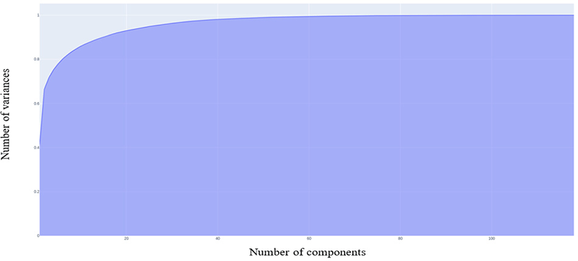
Principal Component Analysis (PCA) is a non-parametric, dimensionality-reduction method. PCA helps to extract relevant information from large datasets by reducing the complexity of the dataset and simplifying the structure [18]. PCA creates new features called Principal Components (PCs). In PCA, initial features are combined to create new features. These new features are uncorrelated. the first components are formed by compressing initial variables which comprise most of the information [12]. For this study, we maintained 99% of the variance and determined the number of PCs required. Fig. 2 shows that 104 PCs are required to preserve 99% of the variance.
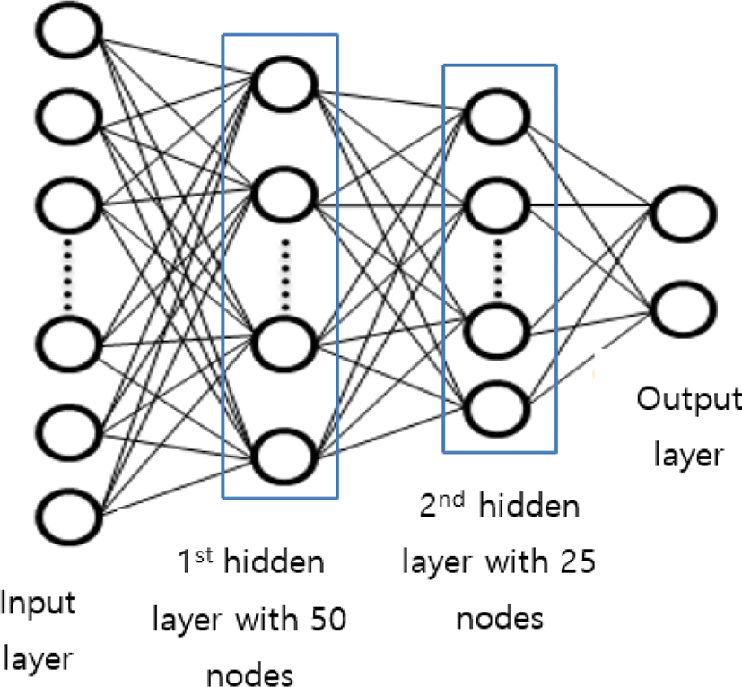
The proposed FC neural network comprises 2 hidden layers. After feature selection, we obtained 104 compressed features. Thus, the input layers have 104 nodes. For the study, we used 50 nodes in the first hidden layer and 25 nodes in the second hidden layer as shown in Fig. 3.
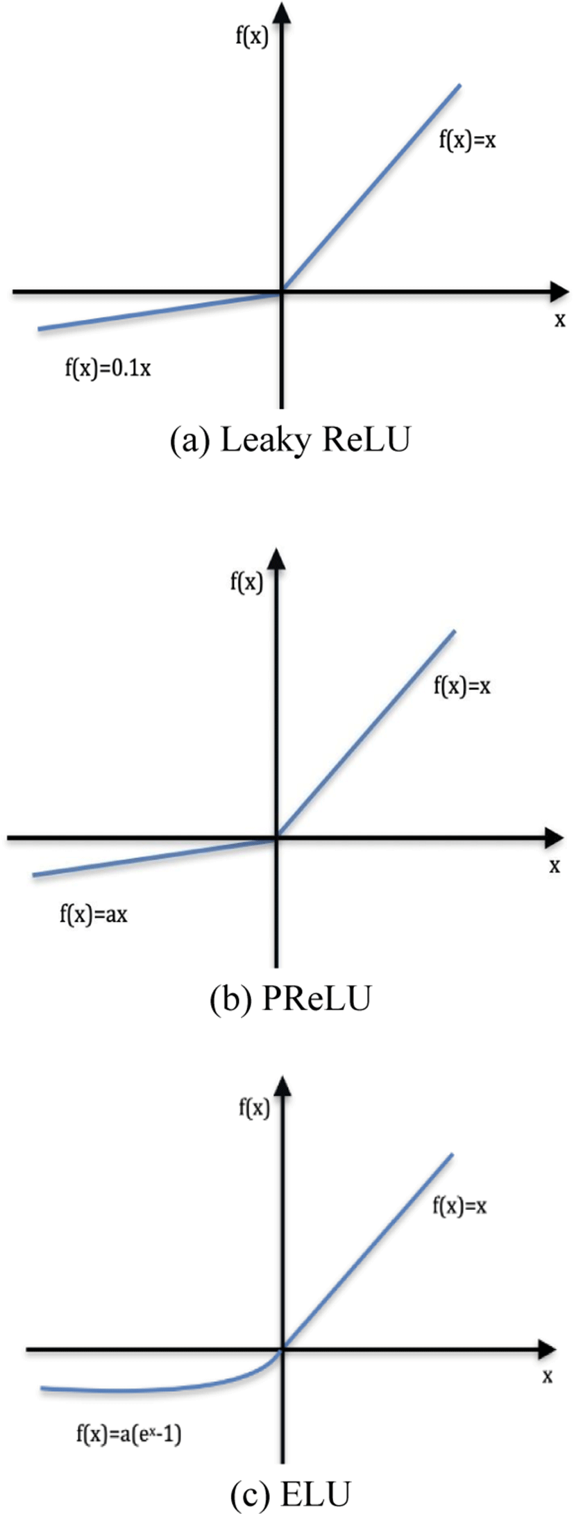
The proposed FC network is built using the Keras library. A combination of three different activation functions was tested. As shown in Fig. 4, these activation functions Leaky ReLU, ELU, and PReLU do not eliminate values for negative values, which overcomes the dying ReLU problem.
For negative values, Leaky ReLU has a slope.
Instead of the fixed slope, PReLU treats the slope as a parameter.
where a is a learnable parameter with a negative slope.
In ELU, a straight line for negative value is replaced by a logarithmic curve. For positive inputs, ELU is similar to ReLU.
III. EXPERIMENT AND RESULTS
For the classification of the test data, there are two parts. The first one is the selection of activation functions based on validation accuracy obtained with these functions. Only training data is used for the validation accuracy. And the second part involves the classification of the test data.
In the validation process, the training data is further divided into two parts: training data and validation data. For this study, we performed three different experiments with ELU, PReLU, and Leaky ReLU in the first hidden layer respectively. Then in the second hidden layer, the same activation functions were used one by one and obtained validation accuracy for a different number of epochs. We obtained validation accuracy for 100, 200, 300, and 400 epochs. Table 4, Table 5, and Table 6 shows the validation accuracy of different FC networks for different epochs.
We performed 5-folds cross-validation. Validation is performed using training data only. Testing data is not used during this process. In this way, we test the model later with the data it has never seen before. Given validation accuracy for each epoch is the average of accuracies obtained from 5-folds cross-validation.
The validation accuracy comparison is performed on the AD vs. CN training data. Comparing the results from the above tables, we can see that the validation accuracy of a model with ELU in the first hidden layer and Leaky ReLU in the second hidden layer has the highest accuracy score of 79.94%. This model is then selected for classification in the next step.
From previous process, a model with the highest score is then used to classify the test data. In our study, we found that the ELU and Leaky ReLU in the first and second hidden layers respectively has better performance than others.
The accuracy (ACC) score of the binary classifier on test data is obtained and then evaluated using a confusion matrix. As shown in Fig. 5(a), four elements of the confusion matrix: true positive (TP), true negative (TN), false positive (FP), and false negative (FN) are used to measure additional performance metrics: sensitivity (SEN), and specificity (SPEC).

For the classification of AD vs MCI, the classifier obtained 83.33% accuracy with 75.00% sensitivity, and 91.67 % specificity. Similarly, for AD vs CN, the scored 87.50% accuracy with 83.33% sensitivity and 91.70% specificity. And for the final classification group; MCI vs CN, the accuracy score was 79.17% with a sensitivity of 100% and specificity of 58.30%.
For the comparison of the proposed model, we used traditional machine learning methods from scikit-learn [19] to classify the same testing data. We used six classification algorithms: Linear Discriminant Analysis (LDA), KNN, NB, Classification and Regression Trees (CART), Logistic Regression (LR), and SVM. We compared the accuracy score, sensitivity, and specificity of these models with the new proposed model.
In AD vs MCI, our proposed network has 83.33% accuracy, which is higher than other listed classifiers. Scores of each model for AD vs MCI is listed in Table 7 and Fig. 6 (a) graphically represented bar graphs of data from the same table. In the case of sensitivity and specificity, the scores are not the highest one but the other classifier which has a higher score in sensitivity or specificity has a lower score in other performance. Like in this case, KNN has the highest specificity but lower sensitivity and accuracy. Our proposed model was able to maintain an almost similar score in all performance matrices along with the highest accuracy.
| Classifier | ACC | SEN | SPEC |
|---|---|---|---|
| LR | 79.20 | 75.00 | 83.33 |
| LDA | 50.00 | 58.30 | 41.67 |
| KNN | 75.00 | 50.00 | 100.0 |
| SVM | 75.00 | 58.30 | 91.70 |
| NB | 41.70 | 41.70 | 41.70 |
| CART | 58.30 | 67.00 | 50.00 |
| Proposed model | 83.33 | 75.00 | 91.67 |
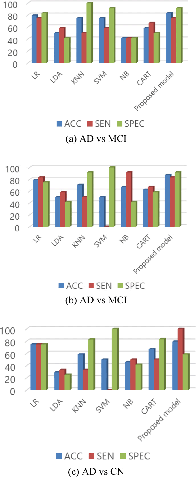
Similarly, in the classification of AD vs CN, the proposed model still scored the highest accuracy of 87.50%. From the data in Table 8 and Fig. 6(b), we can see that the problem with another classifier still remained in this test data as others classifiers could not score high accuracy or maintain the same performance in other parameters too.
| Classifier | ACC | SEN | SPEC |
|---|---|---|---|
| LR | 79.00 | 83.33 | 75.00 |
| LDA | 50.00 | 58.30 | 41.67 |
| KNN | 70.80 | 50.00 | 91.70 |
| SVM | 50.00 | 0.0 | 100.0 |
| NB | 67.00 | 91.70 | 41.70 |
| CART | 62.50 | 67.00 | 58.30 |
| Proposed model | 87.50 | 83.33 | 91.70 |
In the final group, the accuracy is lower than the other two groups but still, it has the highest accuracy than other methods in the group as shown in Table 9 and Fig. 6(c). For MCI vs CN, the model scored 79.17% accuracy. The reason for the poor performance in this group might be because of the reason that there is no vast change in the brain between MCI and CN.
| Classifier | ACC | SEN | SPEC |
|---|---|---|---|
| LR | 75.00 | 75.00 | 75.00 |
| LDA | 29.20 | 33.00 | 25.00 |
| KNN | 58.30 | 33.00 | 83.00 |
| SVM | 50.00 | 0.0 | 100.0 |
| NB | 45.80 | 50.00 | 41.70 |
| CART | 67.00 | 50.00 | 83.33 |
| Proposed model | 79.17 | 100.0 | 58.30 |
The workstation used in this experiment has Intel® Core™ i5-9600K 3.70GHz CPU, 32 GB RAM, and NVIDIA RTX 2070 GPU.NVIDIA RTX 2070 GPU.
IV. DISCUSSION
In this paper, we proposed a novel technique to classify data for the classification of three different groups of AD. In addition, earlier studies aimed to classify using traditional machine learning classifiers and shallow neural networks with the same type of activation functions in layers. In this paper, we studied the combination of different activation functions in the neural network layers. Three activation functions with non-zero values for negative values are considered. The classification validation accuracy of dense neural networks with a combination of PReLU, ELU, and Leaky ReLU are compared.
Many studies have classified the AD groups using different classifiers. However, direct comparison with state-of-the-art methods is difficult as the studies use different modalities and datasets. Comparison with the multiclass classification studies is not suitable for our binary classification model. Classification results in Table 10 compare the proposed model with other studies. The study by Zhang et al. [20] extracted landmark-based features and obtained 83.1% accuracy (80.5% sensitivity and 85.1% specificity) in the classification of AD vs. CN using SVM as a classifier.
| Authors | Classifiers | ACC | SEN | SPEC |
|---|---|---|---|---|
| Zhang et al. [20] | SVM | 83.1% | 80.5% | 85.1% |
| Lin et al. [22] | MLP | 82.86% | 77.72% | 92.31% |
| Zhang et al. [23] | KSVM | 86.71% | 85.71% | 86.99% |
| Chyzhyk et al. [24] | DC | 74.25% | 96% | 52.5% |
| Proposed method | FC-neural network | 87.50% | 83.33% | 91.70% |
The same study obtained classification accuracy of 73.6 %(75.3% sensitivity and 69.7% specificity) for the MCI vs. CN. In another study by Lin et al. [23] used inter-class variance (ICV) for key slices selection and eigenbrain was generated, which was followed by Welch’s t-test (WTT) to obtain most important eigenbrain (MIE) and used kernel-SVMs (KSVM) as a classifier. They obtained a classification accuracy of 86.71% (85.71% sensitivity and 86.99% specificity). A study by Chyzhyk et al. [24], reduced dimension by Lattice Independent Component Analysis (LICA) and used dendritic computing (DC) for binary classification of AD groups. In that study, an accuracy of 74.25% (96% sensitivity and 52.5% specificity) was achieved.
A method similar to our proposed method was used in a study by Lin et al. [22] for the classification of AD groups. A multi-layer perceptron (MLP) of 5 layers with 3 hidden layers classified AD group in that study. However, the features used for the classification are not the same as in our study. Also, the dataset is different and in our study, we maintained a number of subjects to be equal in every group. The study [22] used radial blood pressure waveform (BPW) and finger photoplethysmography signals to train the MLP network and scored classification accuracy of 82.86% (77.72% sensitivity and 92.31% specificity).
Finally, the proposed FC-neural network achieved an accuracy of 87.50% accuracy, a sensitivity of 83.33%, and a specificity of 91.70% for AD vs. CN group. Comparing accuracy scores, our proposed method outperforms other methods listed in Table 10. We also performed a comparison with the state-of-the-art methods using the same data. The results are shown in Table 7, Table 8, and Table 9. Given that the same data are provided to the classifiers, our proposed FC-neural network achieved a higher accuracy score in all three AD groups (AD vs. CN, AD vs. MCI, and MCI vs. CN). Hence, the obtained results from our model are better and comparable to other models.
In Fig. 6, we can see that the sensitivity and specificity of the proposed method is not the best one. We can see that the KNN and SVM has higher specificity. Similarly, LR and NB has higher sensitivity than proposed method in Fig. 6 (a) and (b) respectively. But as we know that sensitivity is obtained from the true positive and specificity is obtained from the true negative predictions. The models which have higher specificity have lower sensitivity, which means that those classifiers were unable to fit the data properly or we can say that it was able to learn from the true negative only which can be interpreted as overfitting for those kinds of data only. In same way, for the classifiers with higher sensitivity, they have lower specificity than the proposed model. This indicates that the models are overfitted with either true positive or true negative only. A model or classifier should be able to classify data properly in different test or group classification. From the Fig. 6, it is clear that the specificity and sensitivity of the proposed model is consistent and doesn’t vary with huge difference for different group classification. This indicates that the proposed model can classify true positive as well as true negative better than other classifiers pointing out that it is the robust in nature than the others.
Recently, there has been significant improvement in the classification using deep learning models. Comparing the results from the machine learning models and the deep learning models, it is clear that the deep learning models are superior to the machine learning algorithms in case of feature extraction and classifications [26-31]. Although, the deep learning process has many advantages over the machine learning, they require huge data to train the model. In deep learning, more the data more better result is obtained. Along with requirement of huge number of data, the deep learning models also require more computational time and better computational setup with graphics processing units (GPU). Our proposed method has advantage of training and testing with comparatively lower number of subjects as well as lower computational time and computational setup.
V. CONCLUSION
In this paper, a binary classifier using dense neural network is proposed. This method alleviates the problem of necessity of multiple modalities and processes. We designed a fully connected dense neural network with two hidden layers to perform binary classification of AD. After comparing the validation of the model with different activation functions in the hidden layers, the model was finalized. The proposed model is compared with six different traditional machine learning methods. Maintaining specificity and sensitivity, the model scored the highest accuracy in all three groups: AD vs CN, AD vs MCI, and MCI vs CN. For AD vs CN, AD vs MCI, and MCI vs CN the accuracy scores are 87.50%, 83.33%, and 79.17% respectively. Finally, we used only T1-weighted images to extract features and after feature reduction, we classified the data with the proposed model. Comparatively, our model does not require a multiple numbers of modalities as input, and multiple models and processes. From the obtained results, we can say that the proposed method with FC model performance is better than other classification methods used for comparison.
Requirement of lower computational time and lower computational setup is the advantage of our proposed model. However, deep learning models have shown more robust and better result in the classification of AD. In our future work, we will implement and classify AD subjects using deep learning models and compare it with the machine learning models. In addition, we aim to use different activation function in deep learning models and get a robust and better classifier.

