I. INTRODUCTION
Learning by supervision means the input is being considered to map some output so that certain characteristics (here class characteristics) are identified/stored in the model. The stored identifying capability can be used for other application (not the one in scratch learning) tasks, which we usually call transfer of knowledge or transfer learning [1-2]. Transfer learning has been a ‘de facto’ savior for most of the state-of-the-art deep learning applications [3-5]. The pretrained weights in the Convolutional Neural Network (CNN) models are finely tuned for the model to be applied in other processes. The major process for this is done by removing the final fully connected layer of 1000 output (for IMAGENET trained models like AlexNet [6], ResNet [7], VGG [8], GoogleNet [9]) into k numbers of output, where k represents the number of labels to be trained in the new task. This implication of the pretrained model into another application not only requires the transfer of weights but also requires the transfer of connection i.e., the whole model trained model is not transferred but just readjusted in its tail part for the new application. On the contrary, with scratch training, we need lots of supervising ground truth and at the same time since the whole network needs to learn from the training material (no external source for learning) it all starts from a ‘zero-level’. And to reach from zero-level to an acceptable ‘fitness’, we need a lot of time, and material and still the acceptable fitness may not be as good as from one already trained model [10].
Krizhevsky et al. [6] successfully utilized CNN in natural image classification (ImageNet Database of 1,000 image types of class) with a minimum error rate in 2012. Later various variants of CNN were proposed by different researchers for image classification and object recognition tasks; the famous ones being Resnet, GoogleNet, and R-CNN [11], etc. Tajbaksh et al. [1] tested CNN in medical images for poly detection and Pulmonary embolism detection, where they highlighted pretrained or fined-tuned CNN performed well as scratch-trained CNN and suggested layer-wise tuning for practical performance. Similarly, Hoo-Chang Shin et al. [12] tested CNN architecture for Lymph-Node detection and Interstitial Lung disease classification, where they also tested a pretrained CNN network (AlexNet, GoogLeNet and CifarNet) and also used the transfer learning technique.
GoogLeNet (also called Inception V1) achieved a top-5 error rate of 6.67% in the ILSVRC competition for the ImageNet classification challenge in 2014 which was very close to the human-level performance. It's an architecture developed by Szegedy et al. [9] at Google Inc. It has 22 layers and adopts multiple parallel convolution layer concatenation which is called the Inception module. The network used a CNN inspired by LeNet but implemented a novel element which is dubbed an inception module. It uses batch normalization, image distortions, and RMSprop. This module is based on several very small convolutions in order to drastically reduce the number of parameters. Their architecture consisted of a 22-layer deep CNN but reduced the number of parameters from 60 million (AlexNet) to 4 million. The key point is that the architecture uses a 1×1 convolution for the ensemble of features. The runner-up at the ILSVRC 2014 competition is VGGNet developed by Simonyan and Zisserman from Oxford University [8]. Out of the six VGG models, VGG16 and VGG19 are frequently used. VGGNet consists of 16 convolutional layers and is very interesting because of its uniform architecture using all 3x3 convolutional filters with stride size 1. The weight configuration of the VGGNet is publicly available and has been used in many other applications and challenges as a baseline feature extractor. However, it consists of 138 million parameters, which can be a bit challenging to handle. This structure is notable for its very simple methodology and has performed well. At last, at the ILSVRC 2015, the so-called Residual Neural Network (ResNet) by He et al. [7] presented a novel architecture with “skip connections” and substantial batch normalization. Such skip connections are also known as gated units or gated recurrent units and have a strong similarity to recent successful elements applied in RNNs. These skip connections also work as a residual connection to preserve the image features by working as an identity function. It achieved a top-5 error rate of 3.57%.
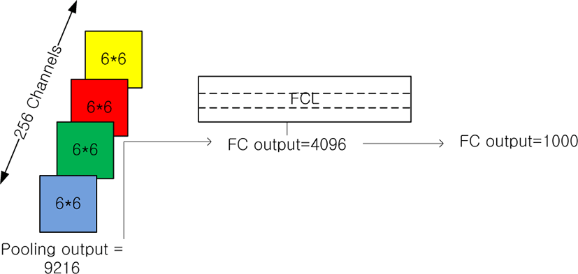
In this research, we are going to reinvestigate the transfer learning process mainly through the weights and feature analysis in the FCL layer. Here the reason for FCL selection is mainly because, of its simplicity and importance for the final decision. Additionally, this is the layer where all the channels/dimension rearranges into two-dimensional feature values [13]. In Section I we discuss the background of research, architecture details of CNN models, and some related work. In section II we discuss the methodology and the user data along with some training procedures. We present our result in section III and provide concluding remarks in section IV.

II. METHODOLOGY AND TRANSFER LEARNING REQUIREMENT
We have used the OASIS dataset brain MRI scans for the experiment. The available MRI scans are in 3D format since the pre-trained models available are only 2D architecture, hence we need to use the 2D images as inputs, for which each MRI scan was converted from analyze format to jpeg format using MRIcon software. Around 30 mid slices were extracted from each MRI scan so in total it produced 840 images each for NC and AD classes. These images were later split randomly in a 5:2:3 ratio for training, validation, and testing as shown in Table 1. All the used MRI scans are made publicly available to download at https://github.com/xen888/Dataset. The reported accuracy is for the 30% test set images. Table 2 shows out of all 3 models, one with freezed weights from the pre-trained model has the lowest accuracy, whereas the accuracy is highest with either fine-tuned or scratch trained. With fine-tuned we can save time, but might not get the best result, with scratch training, we need to train for higher epochs and might get the best result. However, with scratch training, we always have a chance of overfitting the model.
| Class | Total number of scans | Number of scans from single MRI | Total training scans | Total testing scans |
|---|---|---|---|---|
| AD | 840 | 30 | 420 | 252 |
| NC | 840 | 30 | 420 | 252 |
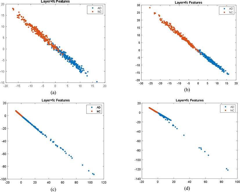
Fig. 2 shows the feature plot of output FCL values (each with 2 scores one for AD and the other for MCI), being plotted in its class label. This plot is not the weights, but the generated value as output from the model. Here each colored dot represents the feature property of an induvial class i.e., blue color for AD MRI and red color for NC MRI.

III. RESULT
Simply, the training and testing result shows that a fine-tuned model works better than a freezed model. However, if we spend more training time, the training will improve the test accuracy at the cost of a higher training epoch.
Table 2 shows the final result of 2D MRI images classification using all three DNN models and trained under three different conditions as below:
-
Freezed: Here the whole network uses the final weights of the pre-trained models, trained on the IMAGENET dataset and as it is available/stored. These weights of all layers are not changed at all during training. A fully connected layer with 2 outputs is replaced with the original final FCL with 1,000 outputs, the input number being the same.
-
Fine-tuned: Here the models have the original weights of pre-trained models as a freezed model. However, during training, these weights are slightly updated using Stochastic gradient descent optimization during backpropagation. Eventually, the weights are slightly tuned for our MRI classification task.
-
Scratch-trained: Here we use the layers of the pre-trained model, but the weights are not transferred at all. It means the model has completely no weights (or say zero weights) before training. Once training starts depending upon the initialization algorithms the weight of each layer gets the value and updates via SGD optimization. Since the layer is weightless at the beginning, its value needs to be learned properly with input values during training hence called scratch training. Here we have used two versions of scratch training, one with a lower epoch e.g., scratch_20 denotes scratch training with only 20 epochs it is done to compare the value of the weight with its freezed and finetuned version. Other is one with a higher epoch to reach full convergence i.e., 100% training accuracy.
The classification performance is shown in Table 2. Here, it is interesting to note that the feature is sparsely dispersion in the case of freezed model and starts to be densely populated in scratch trained model. This might suggest that weights try to converge to a smaller range during scratch training or fine-tuning which is supported by the fact, that the accuracy of freezed model is comparatively lower than other fine-tuned and scratch-trained models (see Table 2). It means when sparsely dispersed the features are difficult to be classified. Also note the difference in the number of parameters i.e., weight values, e.g., in VGG-19 has 4,096×2, here it means 4,096 weights supporting for AD (1st dimension or x-axis) features and other 4,096 weights supporting for NC (2nd dimension or y-axis) features. Here each dimension in the x-y axis corresponds to each class, i.e., the x vs. y plot can be considered as the AD vs. NC plot because the first row of FCL is responsible for making decisions for the AD class and 2nd row is responsible for making decisions for the NC class.
Here more important is the feature distribution pattern as shown in Fig. 2. Fig. 2 shows how the feature distribution varies from complete weight transfer to no weight transfer. Since the freezed model uses pre-trained weights obtained by training from IMAGENET images [14], it is not very supportive for MRI classification (Fig. 2(a)) so, it requires fine-tuning to change the weights to converge into 2 classes properly which is as shown in Fig. 2(b). Fig. 2(c) and Fig. 2(d) show the result of scratch training, features are not properly distinguished and seems condensed with under-training i.e., for only 20 epoch. However, features start to be sparsely distributed under full training i.e., 50 epochs. Similarly, Fig. 3 shows the weight plots of each model. The number of weights for input for FCL is 1,024, 2,048, and 4,096 for GoogleNet, ResNet101, and VGG-19 respectively. With the higher number of inputs being encoded to the smaller output (i.e., 2), we might lose lots of spatial information due to a tremendous reduction in dimension. When using a pre-trained model along with FCL weights we need to condense the high number of input variables into very small output variables equal to the number of classes. As well as the congestion of high input to low output also raises a bottleneck problem, which brings difficulty in encoding and reduces the variability of outputs.

IV. CONCLUSION
In this work, we tried to analyze the class correlation of weights from FCL of various CNN-trained models. This also shows how the architecture plays role in giving classification accuracy along with its length and depth. Consequently, this work is just an attempt to understand how the flattening process works. We tried to analyze the 2D feature distribution process in DNN and besides tried to analyze the weights dispersion pattern. This is an initial work; we hope we can endeavor more understanding of these phenomena in the future.


