I. INTRODUCTION
AD (Alzheimer’s disease) is the most common form of dementia among the elderly [1]. Systematically, it is characterized by the impairment of memory and other intellectual abilities to such an extent that it affects the daily functioning of life. Such neuropathy mainly occurs in the temporal lobe, and a phenomenon accompanied by atrophy of the brain spreads to the entire brain [2-3].
Because the aging brain undergoes atrophy, it is difficult for even experienced radiologists to distinguish between normal age-related atrophy and Alzheimer’s disease-mediated atrophy [4]. Early onset of AD leads to atrophy of the hippocampus. Its dysfunction is believed to underlie the nucleolar features of memory-impaired nitrates [5].
In the case of difficulty in the diagnosis of AD, here comes the true usage of image processing and machine learning. In this context, machine learning models provide great potential to capture even slight tissue alterations [6]. State-of-the-art models for image segmentation and classification are CNNs (convolutional neural networks), which have recently been applied to medical imaging data for various use cases [7].
Specifically, the segmentation of the hippocampus reveals the affected spots of its complex structures and paves a path for the identification of AD. Recently, deep neural networks, and particularly CNN (convolutional neural network), have shown superior performance to other machine learning techniques on computer vision tasks, particularly in semantic segmentation.
The hippocampus has been automated segmented using a variety of algorithms [8-12]. Specifically, HippMapp3r [13], is an open-source, efficient whole hippocampal segmentation pipeline based on 3D-CNNs that is robust to brain atrophy due to neurodegenerative changes.
In case of AD diagnosis, increasing number of algorithms have used 3D convolution for the classification and prediction of AD due to its excellent ability to capture features from spatial information in 3D-MRI (magnetic resonance images). However, the use of 3D convolution increases the computational power requirements. Therefore, this study was aimed at developing a model with a high performance and low computational cost for medical image applications involving SPT (shifted patch tokenization).
The selection of segmenting and classification as based on hippocampal atrophy is due to early onset of AD leads to atrophy of the hippocampus. The training with the less datasets we collected leads to the application of SPT. The overall structure of this research is based on a training and validation with the fewer MRI dataset specific to the AD and to implement the effective model minimize the overfitting with reduced classification error.
In this paper, to implement the pipeline of hippocampus-based AD diagnosis, we segmented a whole hippocampus of the whole dataset through an algorithm based on 3D-CNN (HippMapp3r); The SPT is proposed between the hippocampal segmentation and the EfficientNet application process. It enhances the spatial invariance of the model; This has the effect of increasing the locality inductive bias by embedding more spatial information in each visual transformation. The segmented database was trained and validated through EfficientNet to diagnose deep features and provide a binary classification. The issue of overfitting is minimized with reduced classification error owing to dropout layers. The proposed pipeline delivers an excellent result with higher accuracy as is demonstrated in the confusion matrix.
II. RELATED WORKS
Recently, image classification through CNN models have achieved high accuracy and even exceed the capabilities of human recognition. The neural network focusing on medial temporal lobe including hippocampus provides the earlier diagnosis of AD. The comparison between different CNN models with various techniques has been motioned.
Zhang et al. proposed mask-refined R-CNN to refine the object details in segmentation [14]. In this process, a framework on a mask head is refined and alignment strides are adjusted in the region of interest. Using this process, medical images could also be segmented, and the process was integrated with a CNN named StoolNet [15]. The method proves color classification and maintains a balance between accuracy and computational complexity. As a result of the segmented image classification, more discrimination can be achieved than with the original image.
In earlier stage, the data feed into the 2D-CNN model like Inception-v4 skull-stripped 2D image slices. Continuing with the feature extraction they concatenate the local patient information features with Inception-v4 model features and calculated the cross-entropy loss [16]. Then the multi-model deep CNN for automatic hippocampus segmentation and classification in AD introduced. The 3D-CNNs like RasNet and U-net used for hippocampal segmentation and DenseNet for the features extraction of segmented hippocampus. After, they perform weighted summation on the output features and feed it to the classifier layer [17]. Thus, the multi-model method outperforms the single-model and several other competing methods. To increase the training accuracy by enhancing the hippocampus segmentation, LB (Laplace Beltrami) spectrum with the segmentation tool HippMapp3r were implemented with DenseCNN for classification [18]. This LB spectrum can be calculated by Riemannian manifold as:
where, f is the Riemannian manifold, which is the input for gradient and then divergence. These two types of (shape and DenseCNN features) were expanded and concatenated. This joined trained strategy provides the higher accuracy, but the complex architecture takes too many parameters to train and optimize. Potential features like squeeze-and-excitation module [19]. The upcoming methods like multi-rate signal processing [20] and spatiotemporal learning [21] for the multiple frame approaches are yet to be tested. In that case, the end-to-end deep 3D CNN for the multiclass AD biomarker identification task, using the whole image volume as input with a domain adaptation optimized the one-vs. -rest logistic regression enhanced the target domain and improved the classification probabilities [22].
Since the number of tasks in domain adaptation is huge and optimization algorithm is requiring to speed-up the learning, spatial transformation networks [23] ware introduced to transform the input features into more compact features with fewer parameters than those in standard convolution. Even though these methods improve accuracy, they usually require manual tuning, and still often yield suboptimal performance.
Despite their computational efficiency, these methods are expensive because of CNN complexity, and prone to overfitting because of their high dimensionality. In comparison, the previous classification models based on segmented hippocampus with transfer learning models require a transfer model for every new domain, while the category based on the whole brain might not provide the early stages of atrophy. This indicates the need for SPT to classify hippocampus atrophy more accurately based on different dimensions. The SPT can provide higher accuracy in the network with small data when it is integrated in the pipeline. Furthermore, EfficientNet provides a faster prediction of AD diagnosis than other proposed networks.
III. METHODOLOGY
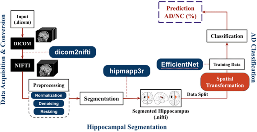
Fig. 1 shows the high-level architecture of the proposed model. The overall pipeline can be divided into three major parts. First one is the data acquisition and preprocessing, second is hippocampus extraction with segmentation network, third is the classification model to classify the AD.
The data used in the study are actual samples collected (during the research project) from medical institutions. T1 weighted three-dimensional volumetric scans of 251 subjects applicable for analysis were generated from MRI brain scan images of 258 subjects [171:NC (Normal Cognitive), AD: 87] and utilized.
The acquisition parameters for the DICOM (Digital Imaging and Communications in Medicine) gradient echo sequence were: +200 slices; matrix. The whole data has the specific manual annotations performed by the experienced physician.
After the data acquisition in DICOM format, we converted the raw DICOM scan slices and then we converted to NIFTI (Neuroimaging Informatics Technology Initiative) the data according to doctor’s annotation and examination and converted the data structure into BIDS (Brain Imaging Data Structure) imaging. This converted and formatted MRI scans have the full head scan.
Prior to training, all images were bias field corrected for B1-inhomogeneities standardized to have a zero mean and unit variance within a local neighborhood of 50 voxels using c3d (Convert3D) tool [24]. We opted for neighbor-hood normalization instead of global image normalization to better preserve local features.
The hipppmapp3r [23] consists of a serial ensemble of two networks, an initial network trained on the whole brain and a second network with the same architecture trained on the first network’s output. It employs skip connections to combine feature maps across stages through concatenation. Every contraction step doubles the number of filters in the network, with a depth of five and 16 initial filters. The building blocks of the networks are convolution blocks, consisting of a convolution layer followed by a normalization layer and a nonlinearity. The leaky ReLU (rectified linear activation unit) was chosen as an activation function with a negative slope of 10−2 for the feature map convolutions [25]. Due to class imbalance data, applied weight map enact to the categorical cross-entropy loss function. HippMapp3r was validated against four other publicly available state-of-the-art techniques (HippoDeep, FreeSurfer, SBHV, volBrain, and FIRST). With an average dice and correlation coefficient of 0.89 and 0.95, HippMapp3r outperformed the other techniques on each metric.
The SPT [26] provides a wider receptive field to the model to be trained with higher accuracy and the effective spatial modeling that tokenizes spatially shifted images together with the input image. The SPT is proposed between the hippocampal segmentation and the EfficientNet application process. It enhances the spatial invariance of the model; This has the effect of increasing the locality inductive bias by embedding more spatial information in each visual transformation. For every given image, the SPT will spatially shift the image in four diagonal directions, that is, up-left, up-right, down-left, and down right. In this paper, this shifting strategy is named S for convenience. The shifted features are cropped to the same size as the input image and then concatenated with the input. As shown in the Fig. 2, This process was done for three dimensions of the MRI image (axial, sagittal and coronal). Spatial shift only by patch-sized clauses in 4 diagonal directions relative to the input image (=S). This can be shown as:
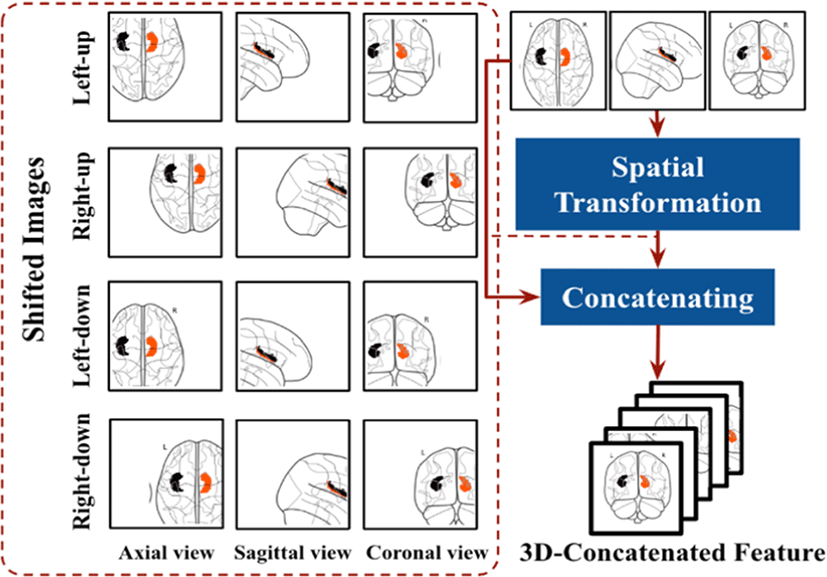
here, sN is shifted images, where P is the concatenation of patches into single image. As a result, SPT can embed more spatial information into visual tokens and increase the locality inductive bias of visual transformation. As a result, the network is fine-tuned to ensure that it achieves maximum accuracy, but it is also penalized if it is computationally intensive.
After the process of image shifting, then concatenate with the given input of the EfficientNet-B0, after the concatenated images divided into non- overlapping patches as standard EfficientNet-B0 input.
CNNs are commonly developed at a fixed resource cost, and then scaled up to achieve better accuracy when more resources are made available. EfficientNet [27], proposes a novel model scaling method that uses a simple yet highly effective compound coefficient to scale up CNNs in a more structured manner. Powered by this novel scaling method and recent progress on AutoML (Automated Machine Learning), they have developed a family of models, called EfficientNets, which super pass state-of-the-art accuracy with up to 10×better efficiency (smaller and faster). The primary step in the compound scaling method is to perform a grid search to find the relationship between different scaling dimensions of the baseline network under a fixed resource constraint [e.g., 2×more FLOPS (Floating-point Operations per Second)] with the parameters of 7.8 million and 0.7 billion FLOPS. MBConv is the main building block of this network, to which squeeze-and-excitation optimization is added. The MBConv algorithm is like the residual inverted blocks used in MobileNet v2. In a convolutional block, they form a shortcut between the beginning and the end. For enhancing the depth of the feature maps, 1×1 convolutions are used first to expand input activation maps.
To reduce the number of channels in the output feature map, 3×3 Depth-wise convolutions are followed by Point-wise convolutions. Shortcut connections connect narrow layers whereas skip connections connect wider layers. As a result of this structure, the overall number of operations is reduced, and the model size is decreased.
As a result of this structure, the overall number of operations is reduced, and the model size is decreased (Fig. 3). This determines the appropriate scaling coefficient for each of the dimensions mentioned above. Then apply those coefficients to scale up the baseline network to the desired target model size or computational budget. Therefore, we can define a CNN layer as:

where denotes the layer Fi is repeated Li times in stage, <Hi,Wi,Ci> denotes the shape of the input tensor X layer i.
IV. EXPERIMENTS AND RESULTS ANALYSIS
Prior to perform AD classification model we performed the hippocampus segmentation and extracted the hippocampus of all the data. The input of the classification network is the output of hippocampus segmentation results.
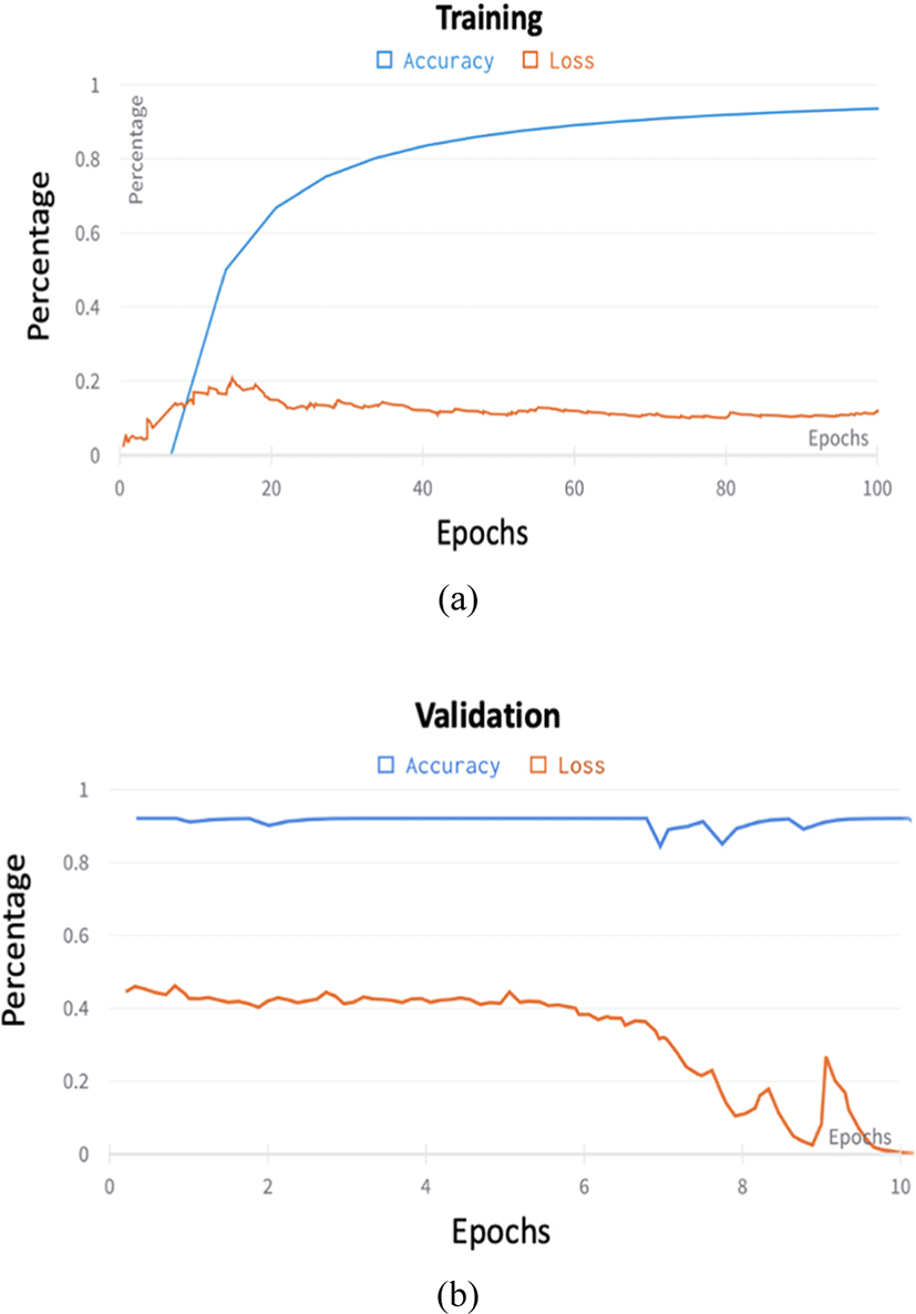
The proposed classification model was trained for 100 epochs and the validation were set to every 2 epochs after. We used the Adam optimizer [28] with an initial learning rate of 1 × 10³, the patience of 100 epochs for the validation loss and a learning rate drop (decay factor) of 0.5. We also use the SiLU activation function from Eq.4. 188 (~70%) were used for training, 64 for testing and 0.9216 for validation during training.
All the network architecture pipeline and their optimization were implemented using compound coefficient, deep learning framework based on Docker container with MONAI (PyTorch-based, open-source framework for deep learning in healthcare imaging), EfficientNet with the python version 3.8 CUDA. For hardware we used the NVIDIA DGX A100 GPUs.
where σ(x) is the logistic sigmoid.
The classification process is fully automatic. The proposed model showed 94% accuracy on training data and 96 % accuracy on the testing dataset. The SPT was effectively improved the locality inductive bias of the training network by increasing the accuracy rate from 87%−94% (Fig. 4). Models like ResNet can be scaled up from ResNet-18 to ResNet-200 by increasing the number of layers. The conventional practice for model scaling is to increase the CNN depth or width arbitrarily or to use larger input image resolution for training and evaluation. Despite improving accuracy, these methods usually require tedious manual tuning and still yield suboptimal results.
To evaluate the proposed model, use three different evaluation measures. First, Sensitivity (equation (5)) is a measure of how well a machine learning model can detect positive instances. The true positive rate (TPR) is also called the recall rate. The sensitivity of a model is used to evaluate its performance because it shows how many positive instances the model was able to correctly identify. Second, Specificity (equation (6)) measures the proportion of true negatives that are correctly identified by the model. Consequently, there will be another proportion of actual negatives that got predicted as positives and could be called false positives. This proportion also be called as True Negative Rate (TNR).
Specifically, each subject was represented as two sets (left/right hippocampus) of three-dimensional objects. The optimizers used to change the attributes of neural networks such as weights and learning rate to reduce losses.
In this experiment, the determination is to provide an optimized treatment to the patient based on the analyzed content. As expected, the EfficientNet provide the best result for the deeper architectures and the threshold of 0.99 was applied to the boundary area detected during the test. We also observed some overfitting in the training data.
However, the performance differences in Dataset between validation and test sets were small, indicating that we appropriately mitigated this problem. In this research, we attempted to classify AD and NC functions based on hippocampus morphological features using machine learning algorithms. It is also proven its usefulness in discriminating.
To verify the superiority of the proposed method, it was compared with the existing methods that reported the binary and ternary classification with higher accuracy. As shown in Table 1, the binary classification performance of the proposed method achieved 96%. Compared to the performance presented in references related to the hippocampal atrophy, the proposed model shows comparatively higher atrophy. Whole brain atrophy classification with CNN and Cam-CNN model performs with better accuracy rates. In case of comparing the hippocampal atrophy and whole brain atrophy classification models, the atrophy in hippocampus with thalamus region shows the early stages of dementia [29]. The preliminary stages of atrophy cannot be identified with higher accuracy by the diagnosis of whole brain. Achieving the highest accuracy using CNN though hippocampus atrophy with small data was a big challenge. Reducing the segmentation and prediction time was hurdled up because it was considered as an important criterion for this pipeline. Choosing the EfficientNet for the robust in transfer learning becomes the important implication for high accuracy with the reasonable amount of computation which includes ~3 minutes for the segmentation process and 0.09 seconds for the prediction of AD using the segmented hippocampus. The reason why the test accuracy is higher than the training set is due to training and validation splitting. Validation examples are small number of data instances compared to training set. We performed training on training data (~74%) and test it few numbers of examples (~26%), due a smaller number of overall datasets. Otherwise, training on dataset with large number of instances and with average splitting of training and testing dataset achieve the balanced accuracy. The SPT provides the efficient amount of data by converting the single image into multiple patches of images. This process becomes the backbone for the higher accuracy in training and validation. Comparing to the previous research on SPT [20] using the spatial transformation outside the training model provides the precise and time-consuming model architecture. Comparing the state-of-art methods mentioned above, our classification model provides the higher classification accuracy in hippocampal atrophy and comparatively higher accuracy with whole-brain and big data like ADNI dependent methods due to the spatial transformation and EfficientNet architecture.
| Author | Processing and training | Classification | Modalities | Accuracy (Eq:7) | Sensitivity (Eq:5) | Specificity (Eq:6) |
|---|---|---|---|---|---|---|
| Basaia et al. (2019) [30] | Whole Brain | CNN |
AD-NC, AD-MCI, MCI-CN |
99.21) 75.487.1 87.7 |
98.9 74.5 87.7 |
99.5 76.4 74.6 |
| Wang et al. (2021) [31] | Hippocampus-based biomarker | Dense CNN | AD-NC | 89.8 | 98.5 | 85.2 |
| Liu et al. (2019) [16] | Segmented hippocampus | Multi-model CNN | AD-NC | 88.9 | 86.6 | 90.8 |
| Katabathua et al. (2021) [15] | Hippocampus atrophy | DenseCNN2 | AD-NC | 92.5 | 88.2 | 94.9 |
| Zhang et al. (2021) [32] | Whole brain | CAM-CNN | AD-NC | 97.3 | 97.1 | 99.7 |
| Proposed method | Hippocampus atrophy | Efficient Net | AD-NC | 962) | 96.9 | 100 |
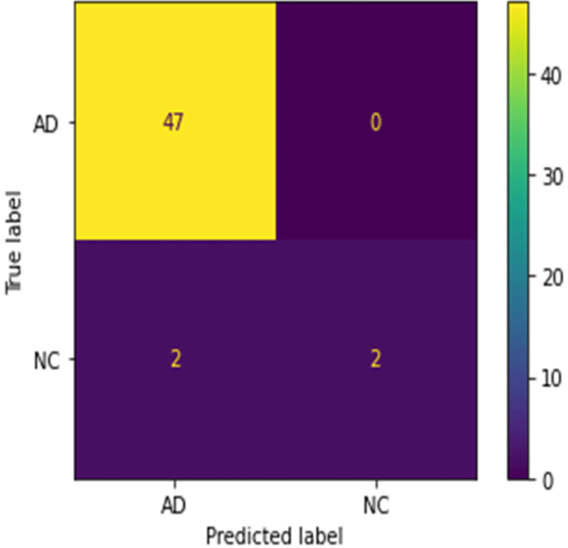
There are separable convolution layers in depth to reduce the number of parameters and computations to a smaller extent. It is possible to achieve excellent classification accuracy using EfficientNet. It obtains deep image information and reconstructs dense segmentation masks for brain classification of AD with NC (Fig. 5).
The performance of the network was tested using pre-processing, SPT, and classification on T1 weighted MRI. Comparison between the proposed approach and existing deep learning methods shows a higher classification accuracy. The reason for adding more AD data is the data contains more early stages of AD and brain atrophy called MCI (Mild Cognitive Impairment). It is a challenge to diagnose the early stage of AD. As the correlation between the true label and the predicted label for AD and NC is 0, we assume that the classification model predicts the AD even in early stages. In that case, the small data of NC may not lead to the model bias. Despite requiring fewer training samples, it delivers excellent results as is demonstrated in the confusion matrix. By reducing classification errors due to dropouts, overfitting is minimized.
V. CONCLUSION
In this work, the hippocampal segmentation and AD-NC classification using 3D-CNN is proposed. The U-Net model was found to be able to extract the voxels of hippocampus and the EfficientNet provides the higher classification accuracy for AD-NC. Integrating the SPT in the pipeline allows the network to provide the higher accuracy with the small data. It has also been found that the EfficientNet provides the faster prediction of diagnosing the AD comparing other network proposed. In future aspects, we try to make the model to provide its full potency in few iterations [15].
To implement the diagnostic model into a commercial scale, the package will be built and introduced as a software and a mobile application. This will provide fast and easy access to the patients to overview the AD diagnosis. In this context, we can bale to provide an end-to-end pipeline for the classification of AD with higher prediction value which will assist the physicians and the experts to diagnose the Alzheimer’s Disease.

 received his Ph.D from Korea Maritime and Ocean University, South Korea in 2020. His area of expertise is molecular biology and biotechnology. Presently, he works at Unomic Ltd as a senior researcher in the bio and health care division. In addition to metagenomics and transcriptomics, he has a strong interest in Next Generation Sequencing, Deep Learning, and Bioinformatics.
 received his B.S. and M.S. degrees in the Department of Computer Science and Engineering from COMSATS University Islamabad, Pakistan. He received his MS degree from Chung-Ang University Seoul, Korea with Department of Computer Science and Engineering, in 2019 and 2022, respectively. His research interests include image coding algorithms, video coding technique and depth estimation algorithms in stereo vision.
 received his B.S. and M.S. degree form Kyungsung University, Korea, in 1997 and 1999. He received his Ph.d degree in the Department of Information and Communication Engineering from the University of Pukyong National University, Korea, in 2014. He has been a member of IEEE since 2000. His research interests include protocol engineering, big data analytics with machine learning, and Industrial IoT.
 received the M.S. and Ph.D. degrees in the Department of Information and Communication Engineering from University Paris Diderot in 1990 and 1993 respectively. Currently, he is a Professor in the Department of Information and Communication Engineering at Pukyong National University. His research interests include wireless network security technology, transmission network and access network technology, IoT, and big data analytics with machine learning.