I. INTRODUCTION
The introduction of AI, which is available in reality, is expected to have a lot of influence on human life. However, its effect is difficult to expect a positive impact in all fields. It will have a positive impact on productivity or some occupations, but it may have a negative impact on some jobs. It is not the first time. When new technologies or concepts in most of fields were introduced, both positive and negative impacts occurred at the same time: TV, radio, internal combustion engine, aircraft, mobile phone, smart-phone, computer, robot, business process reengine-ering, big data. Some technologies have matured enough and have already had a lot of influence on us, and some technologies are still initial.
A lot of firm-level studies have generally found a lot of positive effects of IT. Case studies on companies that had a positive effect by using IT properly have made many executives interested in IT and willing to invest in IT. In addition, companies that have invested more IT compared to competitors were able to achieve better performance than competitors [1-5]. Considering the appropriate investment on supplementary assets, the strong relationship between IT investment and economic performance was more easily found.
In the studies using cross-sectional data that considers a competitive environment, the positive effects of IT were found regardless of the level of analysis of companies (e.g., [1-5]), industries (e.g., [6]), and countries (e.g., [7-8]). Many studies have found that if the company or country invests more IT investment than competitors, they can make better performance than competitors. Of course, the study that did not find the positive effects of IT is generally not easy to be published in IT-related academic journals.
In terms of a single industry (e.g., NAICS (North American Industry Classification System) 334, Computer and electronic products manufacturing) or a single country (e.g., Unites States) that is not in a competitive environment, a longitudinal study using time series data investigates that more IT investment in a single industry or country will make better economic performance. In general, economic achie-vements of industries and countries are measured using value added or Gross Domestic Product (GDP).
GDP is the sum of the value added by industry. The effect of country-level IT investment on GDP may not be simple. Autonomous vehicles consisting of various sensors incl-uding IT will have a significant impact on human movement and economy. Autonomous vehicles use many electronics products, so it will increase the value added of Computer and electronic products manufacturing industry. However, the expansion of the sharing economy using autonomous vehicles can reduce the desire of ownership of automobiles, the value added of the automobile manufacturing industry (NAICS 3361-3363, Motor vehicles, bodies and trailers, and parts manufacturing), or the car and parts dealer retailers (NAICS 441000, Motor vehicle and parts dealers) can be reduced. In addition, the value added of Truck transportation industry (NAICS 484), which uses autonomous trucks that do not require truck drivers, can be reduced. Internet banking, AI, automotive sharing model, and OTT (over-the-top), which actively utilize IT, are in similar situation. The value added in specific industries increases, but the value added in other industries can be reduced. It may not be clear whether the economic performance of IT will increase or decrease at the single country.
After the existing research (e.g., [9]) using the US time series data, significant events such as the 2008 global financial crisis (GFC) and Covid-19 pandemic (2020) have had a significant impact on the global economy. Many countries tried to overcome the crisis with quantitative easing, and the concepts and trends of the economy were also changed. Considering that the price of computer hardware with the same performance every two years was falling to half, the effect relationship of IT on economic performance can be changed. Moreover, existing research (e.g., [9]) have limitations considering excessive maximum time lags. In addition to the risk of overfitting, the economic performance of eight years ago is too long to affect the current IT investment.
The remainder of this paper is organized as follows. First of all, the studies that analyze the relationship between IT and economic performance and the studies using the Granger causality model are briefly reviewed. The research method and data section described the Granger causality model and data. The result of empirical analysis is explained in the results section. The conclusion section shows the research summaries, contributions, limitations, and the directions of future research.
II. BACKGROUND
Many researchers were interested in measuring the effects of IT investment and conducted research using various sources and analysis methods. Many studies have found positive achievements from IT investment [1-5,10]. These studies have been carried out at the level of enterprise in the competitive environment because of the ease of collecting data. When country-level economic performance is calculated by aggregating the performance of industries that are differently affected by IT, it may not be possible to find a positive impact at the country level that is not under competitive environment.
Table 1 is a part of existing researches by direction of effect in IT and economic performance and analysis level. Further review of existing researches is to refer to the existing studies that analyze the relationship in IT investment and economic performance (e.g., [9-10,22-23]).
| Direction | Level | Existing research and its result |
|---|---|---|
|
IT affects economic performance (IT → EP) |
Firm |
Brynjolfsson and Hitt [1]: P Kohli, Devaraj, and Ow [2]: P Lee and Kim [3]: P Mithas and Rust [4]: P Saunders and Brynjolfsson [5]: P Chae, Koh, and Prybutok [11]: NS |
| Industry | Cheng and Nault [6]: P | |
| Country |
Dewan and Kraemer [7]: P Park, Shin, and Shin [8]: P |
|
|
Economic performance affects IT (EP → IT) |
Firm |
Hu and Quan [12]: NS Kobelsky, Richardson, Smith, and Zmud [13]: P Mitra [14]: P |
| Industry | Gurbaxani [15]: P | |
| Country |
Gurbaxani [15]: P Shih Kraemer and Dedrick [16]: P |
|
|
Bidirectional, granger causality (IT ↔ EP) |
Firm | Hu and Plant [17]: P |
| Industry |
Hu and Quan [18]: P Lee and Ryu [19]: P Lee [20]: P |
|
| Country |
Lee and Kim [9]: P Lee and Ryu [19]: P Lee Ryu and Kim [21]: P |
This table is from Lee [20] with adding some existing studies. EP means economic performance, P and NS means positive and not significant, respectively. The table included only a part of the existing research.
In general, in the field of natural sciences, the causal relationship can be proved by comparing the treatment group, which affected by cause in a strictly controlled environment, and a control group that does not affected by cause. The A/B test for changing the screen design in web page is similar. However, in the field of social sciences analyzing economies or natural sciences such as climate research, it is not easy to find a causal relationship because it is difficult to conduct repeated experiments in a controlled environment such as a laboratory [24]. In order to analyze the causal relationship between carbon dioxide concentration and temperature, carbon dioxide concentration cannot be increased or the temperature of the earth cannot be operated. Or it is difficult to artificially change the economy to analyze whether economic growth affects IT investment. It is necessary to try to find causal relationships using statistical methods that use the already accumulated available data, rather than acquiring data through experiments. The researchers can find the economic situation, which is similar to the experimental envir-onment, by chance or in-depth exploration [25], and use the Granger causality model [26].
The Granger causal model is used in various fields of research. Economic growth and government fiscal activities [27], population [28], trade [29], tourism [30], export/ imports [31], underground economy [32], Defense spending [33], health care spending [34], female labor participation [35], communication technology investment [24,36-37] were analyzed. Moreover, it has been used in various economic situations such as the football team's performance and revenue [38], inflation and unemployment rate [39], IT investments and employment [40], cryptocu-rrency uncertainty and crude oil and gold prices [41], airport and regional economic growth [42].
In addition to the economic situation, other phenomena such as the AI index and carbon prices [43], temperature, carbon dioxide, methane [44], the phenomenon in which the temperature of the Northern Hemisphere of the Earth rises first and the temperature of the Southern Hemisphere rises later, but the temperature of the Northern Hemisphere does not rise even when the temperature of the Southern Hemisphere rises [45], and political and diplomatic situations where Israel responds to Palestinian violence with violence, but Palestinians do not respond to Israeli violence [46] were used. Although it is difficult to perform artificial causal experiments, the Granger causality model were widely used if researchers could secure sufficient time series data for analysis by monthly/quarterly or long-term data.
The results of the studies analyzing the Granger causality relationship between IT investment and economic performance can be referred to existing studies (e.g., [19]). The Granger causality model was widely used in a variety of fields, but limited in IT-related academia. IT research with the cross-sectional data has been more active in rather than longitudinal data, may be partially due to the rapid change of IT. If appropriate time series data can be secured, research methods need to be expanded [47].
III. RESEARCH METHOD AND DATA
The Granger causality model is a method that generally uses two time series data to investigate the relative changes between the time series over time [20,26,48]. The following two equations are used to determine whether X has a Granger causality effect on Y:
where Yt−i is Y at time t−i, Xt−i is X at time t−i, αi and βi are regression coefficients, k and l are lags, c1 and c2 are constants, and ε1t and ε2t are error terms.
If the significance of the regression model in equation (1) is satisfied and αi is statistically significant, it shows that the current Y can be explained or predicted by the past Y. Equation (1) is a forecasting model that can be used to explain the current state or value using past data [26,49].
The Granger causality model compares equation (2), which added Xt−i, to equation (1). If equation (2) is significantly superior to equation (1) (or βi is statistically significant), it can be interpreted as X has Granger causality on Y [26]. If the addition of X to the regression equation improves the explanatory power of the regression model, then X is an explanatory (independent) variable that influences Y. If the explanatory power of the model does not improve even though X is added to the regression equation, it can be interpreted that X does not have Granger causality on Y. In addition, the sign and statistical significance of determine whether the effect is positive, negative, or non-causality. The statistical superiority of equations (1) and (2) is compared using the following equation [49-50]:
where RSSr is the residual sum of squares in equation (1), RSSu is the residual sum of squares in equation (2), w=(M−r)−(N−s), M is the number of observation in equation (1), r is the number of coefficient in equation (1), N is the number of observation in equation (2), and s is the number of coefficient in equation (2).
If the F-test statistic calculated by equation (3) is greater than the critical value of the F-distribution with the degrees of freedom (w) in the numerator and the degrees of freedom (N−s) in the denominator, then equation (2) is statistically superior to equation (1), and therefore X is a statistically significant independent (explanatory) variable that affects Y. A statistically significant βi indicates the Granger causality of X on Y.
This study analyzes the causality between IT capital and economic performance in the US private business sector using production function theory and the Granger causality model. Studies using production function theory view the factors of the production function as IT capital, non-IT capital excluding IT, and labor, and they try to find that an increase in IT capital increases production quantity more efficiently [1,6,19-20]. Many researches used the growth rates of IT capital and value added (e.g., [51]) due to the stationarity of the data described below. To determine whether IT capital has a causal effect on economic performance, we apply the growth rate of the IT capital to the X in equations (1) and (2), and the growth rate of the value added to the Y in equations (1) and (2).
Economic performance is a determinant of IT investment, and abundant economic performance increases IT investment, which in turn increases IT capital [15]. To determine whether economic performance has a Granger causality on IT capital, we apply the growth rate of the value added to X in equations (1) and (2), and the growth rate of the IT capital to the Y in equations (1) and (2).
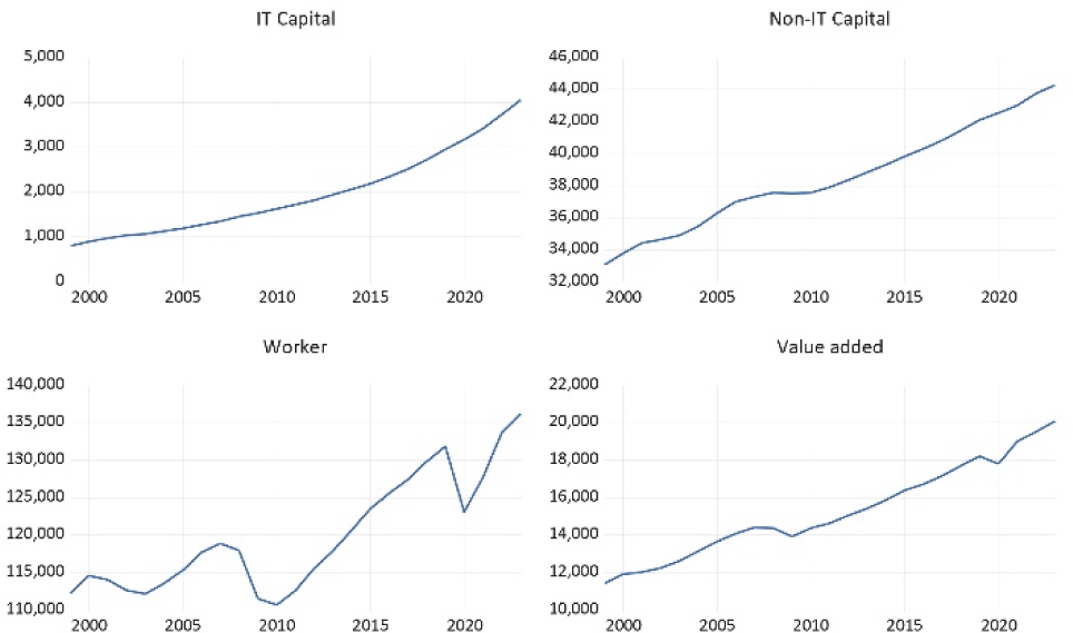
In analyses with time series data, such as Granger causality analysis, it is necessary to check the data’s stationarity that the statistics such as mean, variance, and covariance are not changing and depending on the flow of time. The analysis using non-stationary data can produce spurious regression results, distorting the analysis results [49]. In this study, data stationarity was verified using the Breakpoint Unit Root Test, which accounts for structural changes in time series data [52]. Looking at the IT capital and non-IT capital in Fig. 1, the mean increases over time, indicating that the data may not be stationary. The precise results can be confirmed in the unit root test results. EViews 12 was used as the analysis tool.
Next, we need to determine which lag (k, l) of the regression equation for Granger causality is most appropriate. If a theory related to the optimal lag is already established, it can be determined based on the theory. However, if there is no theory regarding optimal lag, the data can provide it. Among various lag models, the lag of the model with the smallest Akaike Information Criterion (AIC) can be considered the optimal lag [49-50]. In addition, Granger causality analysis basically uses regression analysis. In regression analysis, the number of observations must be at least five times the number of independent variables to avoid overfitting [50, p. 166]. Considering the number of observations in the current study (N=25) and the number of explanatory variables in equation (2), the maximum lag is only two years.
The capital used in this study is from the Bureau of Labor Statistics (BLS) [53], while the number of workers and value added are data published by the Bureau of Economic Analysis (BEA) [54]. IT capital is calculated by adding software (the software category of intellectual property products) to information processing equipment, which is composed of computers, communications, and other information processing equipment, in the BLS's capital classifycation. Non-IT capital is calculated by subtracting IT capital from capital.
As of 2025 the data from 1999 to 2023 are available period for all variables including the growth rate. This study focuses on the private business sector excluding the government sector since decision-making methods for investment in the government sector, which is operated with the tax, may differ from those of the private business sector.
IV. RESULT OF ANALYSIS
Fig. 1 shows IT capital, non-IT capital, number of workers, and value added by year in US private business sector. IT capital has steadily increased, while NIT capital has grown linearly, except for a period of stagnation during the 2008 GFC. The number of workers has increased, but decreased during the dot-com bubble burst (2000), the 2008 GFC, and the COVID-19 pandemic (2020). The value added has shown a continuous increase, except for a period of stagnation during the dot-com bubble burst and a decrease during the 2008 GFC and the COVID-19 pandemic.
Fig. 2 is a cumulative graph of IT capital, which is composed of computers, communication, software, and other information processing equipment. While computer hardware shows relatively slow growth, software and communication show relatively rapid growth, steadily increasing their share of IT capital. Current investment for IT is mainly related to software and communication.
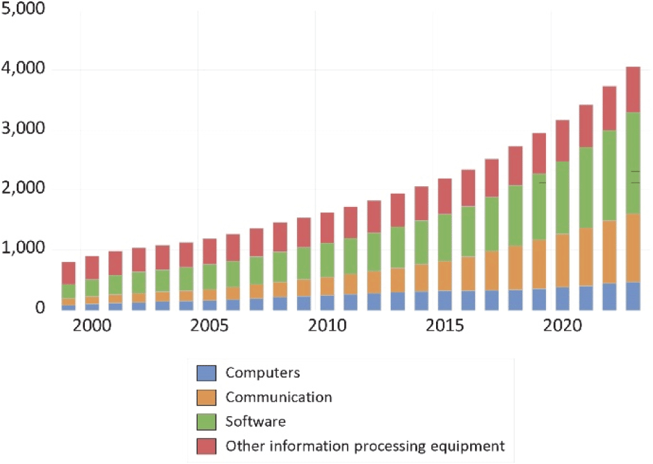
The proportion of software and communications in IT capital composition shows an increasing trend, while the proportion of other information processing equipment decreased from about 50% to about 20%. This suggests a growing importance of software, as well as the increasing importance of communications that connect computers.
Fig. 3 shows individual graphs of computers (hardware), software, communication, and other information processing equipment. Computers and other information processing equipment increased linearly, while software and communications grew exponentially. This may be due to the recent increase in the importance of software and communications within IT capital, or the long depreciation period of software and communications equipment, allowing for long use.
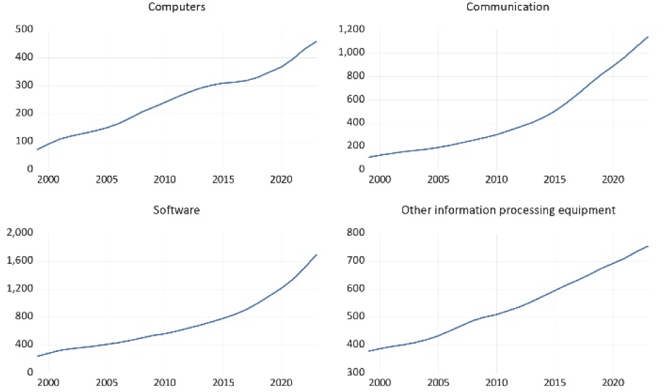
Fig. 4 shows the growth rates of IT capital, non-IT capital, number of workers, and value added. IT capital is showing a high growth rate of over 4 percent. The growth rate of non-IT capital is around 1 percent. The growth rates of the number of workers and value added show similar trends, they experienced negative growth during the 2008 GFC and the COVID-19 pandemic.
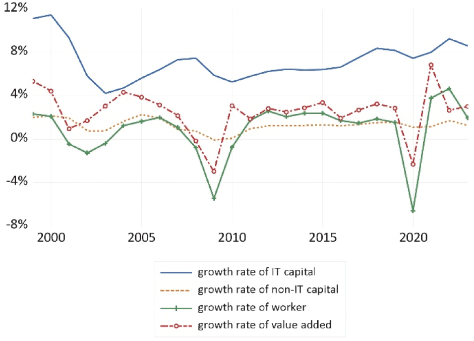
Fig. 5 shows the growth rate of IT capital per worker, non-IT capital per worker, and value added per worker. During periods of declining employment (Fig. 1), capital per worker and value added per worker show a spike in growth. While the growth rate of IT capital per worker is over 4%, non-IT capital per worker has barely increased since 2011 excluding the COVID-19 pandemic period, which shows a significant number of layoffs.
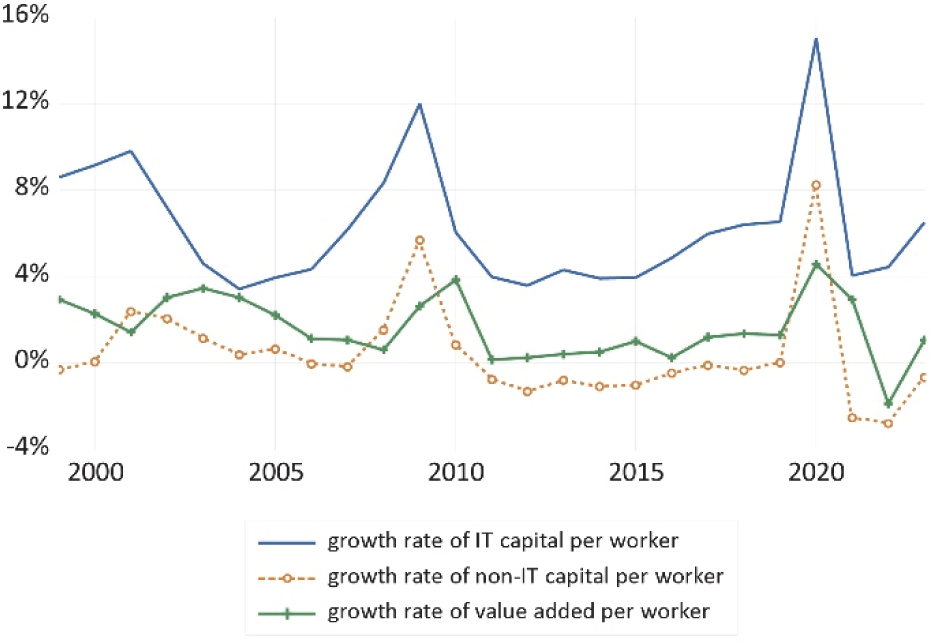
Table 2 presents descriptive statistics. The average IT capital is $ 1.96 trillion, the minimum is $ 798.9 billion (1999), and the maximum is $ 4.06 trillion (2023). The average non-IT capital is $ 38.48 trillion, with a minimum of $ 33.06 trillion and a maximum of $ 44.28 trillion. The average annual value added is $ 15.27 trillion, with a minimum of $ 11.43 trillion and a maximum of $ 20.09 trillion. The average annual number of workers is 119.89 million, with a minimum of 114.27 million and a maximum of 136.27 million. The average annual IT capital per worker is $ 16 thousand, non-IT capital is $ 320.7 thousand, and the value added is $ 126.7 thousand.
The average growth rates of IT capital, non-IT capital, number of workers, and value added are 7.2%, 1.3%, 0.9%, and 2.5%, respectively. Minimums of the all variables except IT capital were negative that means a decrease. The average growth rates for IT capital per worker, non-IT capital per worker, and value added per worker were 6.3%, 0.4%, and 1.6%, respectively. Their maximums are 15.0%, 8.2%, 4.6%. Their minimums are 3.4%, −2.8%, −1.9%. IT capital consistently increased throughout the analysis period, but other variables did not.
The Breakpoint Unit Root Test using the Augmented Dickey-Fuller (ADF) revealed that IT capital, non-IT capital, number of workers, and value added were non-stationary, but their growth rates were stationary. The graphs in Figs. 4 and Fig. 5 show the stationarity of data, while plots in Fig. 1 show non-stationary data.
Table 3 shows the results of the Granger causality analysis. The optimal lag was selected as the lag with the smallest Akaike Information Criterion (AIC). The growth rate of IT capital did not show Granger causality on the growth rate of value added (F value=0.7). This means that even if IT capital increases, value added does not rise. This may be due to the productivity paradox of IT [55], which states that national economic growth may not increase despite an increase in IT capital. While IT capital may play a significant role in economic growth in information intensive industries such as the electronics industry, it may not play a significant role in economic growth in less information intensive industries such as agriculture, forestry, and fisheries [3]. Furthermore, IT capital may have no effect at the national level since the effects of IT in individual industries are mixed.
| Direction of causality | Optimal lag (k, l) | F value in equation (3) | Result |
|---|---|---|---|
| GIT → GVA | 1, 1 | 0.7 | - |
| GVA → GIT | 2, 2 | 2.1 | - |
| GIT → GW | 1, 1 | 1.0 | - |
| GW → GIT | 2, 2 | 2.2 | - |
| GPIT → GPVA | 1, 1 | 8.1*** | Positive (+) effect, statistically significant |
| GPVA → GPIT | 1, 1 | 3.3* | Negative (−) effect, statistically significant |
The growth rate of value added also did not show Granger causality on the growth rate of IT capital (F value =2.1). This means that even if economic growth creates the capacity to invest in IT, it does not automatically lead to increased IT investment. Ultimately, while investment capacity is important, this may be because investments are made based on expected future returns.
IT capital can change the production factors involved in production. Even if a restaurant introduces a robot for food delivery, it is unlikely to increase the number of customers. Restaurant owners consider introducing robots to reduce labor costs rather than increase sales. Similarly, ordering kiosks in restaurants and cafes are introduced to reduce labor costs rather than increase sales.
IT can reduce the number of workers, which is one of production factors [20]. However, there is no causality between the growth rate of IT capital and the growth rate of the number of workers since F values (1.0, 2.2) are not significant. The result of country-level analysis can be different from existing research (e.g., [20]) focuses on information intensive industries such as electronics manu-facturing.
IT can increase labor productivity, not output (value added) [20]. Granger causality analysis was conducted using IT intensity (IT capital available to one worker) rather than the total amount of IT capital, and the value added produced by one worker rather than the total value added. The growth rate of IT capital per worker shows Granger causality on the growth rate of value added per worker (F value=8.1***, statistically significant at the 1% level). Increased IT capital increases labor productivity, which is output per labor input. Fig. 5 shows that the change in the growth rate of IT capital per worker moves ahead of the change in the growth rate of added value per worker. In the results of the causality analysis in the opposite direction, the growth rate of value added per worker shows weak Granger causality on the growth rate of IT capital per worker (F value=3.3*, statistically significant at the 10% level). However, the direction of the effect is negative. Although its statistical significance is weak, the growth rate of value added per worker decreases the growth rate of IT capital per worker.
The growth rate of IT capital per worker and the growth rate of value added per worker do not form a virtuous cycle in which they continuously increase while influencing each other. An increase in IT capital per worker increases labor productivity, and increased labor productivity decreases the growth rate of IT capital. A decline in the growth rate of IT capital reduces labor productivity, and this decreased labor productivity, in turn, increases IT capital.
According to production function theory, which considers capital (including IT) and labor as factors of production, capital can substitute for labor, and labor can substitute for capital. Corporate executives determine the optimal combination of production factors by considering the costs and expected performance of capital and labor. If labor costs increase due to rising wages or capital costs decrease by new technology, they seek to replace labor with capital. IT-controlled mechanical devices that can replace labor are readily observed. They may be ordering kiosks in restaurants, automated warehouse systems (robots) in logistics companies, unmanned convenience stores like Amazon Go, automation/mechanization of manufacturing production lines, mobile banking and transactions in financial institutions, mobile check-in systems using websites or apps in airlines, and self-check-in systems where passengers use kiosks at airports. Recently, AI is beginning to influence humanity. Corporate executives can make decisions to maintain a high growth rate of IT capital and a low growth rate of workers to increase labor productivity (Fig. 4). This can forecast a potential decline in labor demand brought about by the Fourth Industrial Revolution [20] and AI.
V. CONCLUSION
An increase in IT capital did not boost national-level economic growth that measured by value added. At the national level, the effects of IT may be mixed, as some industries where IT promotes value added creation, while others do not [3]. This may be why we failed to find that increased IT at the national level boosted value added. However, an increase in IT capital per worker (IT intensity) boosted value added per worker (labor productivity). IT can increase labor productivity regardless of whether IT contributes to economic growth within each individual industry. The finding that IT increases labor productivity is consistent with previous studies. Utilizing IT can achieve the same output with less labor, or even greater output with the same labor input.
Current study has some contributions. First, this is method extension analyzing situations or phenomena similar to previous studies using a different research method [47]. They are usually cross-sectional analyses that companies or countries using more IT than their competitors achieve better economic performance (e.g., [1-8,10]). However, this study presents a time series analysis of the impact of increased IT capital on value added and labor productivity in a single country. This can contribute to theory-building by generalizing research findings aimed at analyzing the economic performance of IT.
Causality requires the following three conditions to be satisfied [56]: (1) association—a connection between cause and effect, (2) temporal precedence—the cause occurs tem-porally before the effect, and (3) isolation—no third factor exists between the cause and effect. The finding of this study is not based on correlation analysis, which satisfies association, but rather on the Granger causality model, which considers association and temporal precedence. Even if Granger causality exists, causality may not exist, but if Granger causality is not found, causality is absent.
Second, this study is context extension investigating similar situations or phenomena using data different from those of previous studies, and can contribute to the generalizability of research findings [47]. Unlike previous studies (e.g., [1,3,6-7]), the current study is the result of an analysis using the most recent data (1999–2023) that reflects the dot-com bubble burst, 2008 GFC, COVID-19 pandemic, and recent rapid development of IT, which had a significant impact on the US economy.
Like most studies, this study has limitations. First, the Granger causal model, which utilizes two time series data, satisfies association and temporal precedence, which are the necessary conditions of causality, due to production function theory and the characteristics of model. However, it could not control (isolate) third factors (e.g., economic cycles) that may influence both IT capital and value added at the same time. Previous studies (e.g., [9,16,24,36]) have also struggled to address this third factor issue. This may be due to the limitation inherent in economics that is hard to conduct experimental studies, which compare outcomes between intervention group and control group. Since the current study utilizes annual data with a limited number of observations, it is hard to control for third factor such an economic fluctuation. The Granger causality model fundamentally relies on regression analysis, to avoid overfitting, the number of observations must be at least five times the number of explanatory variables [50, p. 166]. This study has 25 observations, but even with the maximum time lag of two years in equation (2), there are already four explanatory variables. The limited number of observations makes it difficult to add control variables.
Second, the analysis results are based on US data. The US possesses high IT intensity and sufficient complementary assets, as noted in previous studies, which may limit the generalizability of the results. However, few countries can provide time series data as reliable as the US. The Granger causality model requires long-term time series data.
Third, while increases in IT capital may have long-term effects (e.g., three years or more), the limited maximum time lag (two years) had to be considered in this study. This limitation stems from the insufficient number of observations. In equation (2), the number of explanatory variables is twice the maximum lag. On 25 observations, the maximum possible lag without overfitting is two years.
Future research is needed to address the limitations of the current study. Third factors such an economic fluctuation that may influence both IT capital and value added at the same time, should be controlled. Of course, increasing the number of observations using long-term data or quarterly or monthly data is necessary. Increasing the number of observations not only controls for third factors but also increases the maximum possible time lag. Furthermore, for generalizability of the research results, analysis at the level of countries other than the US or individual industries could be considered. In addition to analyzing the impact of IT in highly information intensive industries (e.g., the electronics industry [20]), the impact of IT in less information intensive industries (e.g., agriculture, forestry, and fisheries) should also be analyzed.