


I. INTRODUCTION
Feature extraction and feature selection are the key criteria in classification and pattern recognition problems. This is greatly useful in the large dimension of input data cases. In recent years, interest in tensor decomposition is gotten more attention from many researchers from various fields. Tensor decomposition is a method to divide a tensor in multidimensionality into many smaller parts. Two well-known methods in this area are CANDECOMP/PARAFAC (CP) decomposition and TUCKER decomposition. Both CP decomposition and Tucker decompositions can be considered as higher-order generalization of Singular value decomposition (SVD) and Principle Component Analysis (PCA) [4]. These methods are always used to decompose data into simpler form, containing better features. Decompositions of tensor have applications in various fields: data mining, neuroscience, graph analysis, computer vision and elsewhere. This paper gives an application of tensor decomposition into EEG signals.
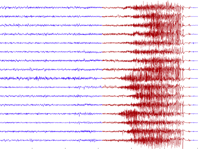
Electroencephalography (EEG) is a kind of the brain data. It is a measurement of many brain signals which are recorded from a number of electrodes placed along the scalp. More clearly, EEG is the recording of electrical activity along the scalp. It measures voltage fluctuations resulting from ionic current flows within the neurons of the brain. In clinical contexts. EEG refers to the recording of the brains spontaneous electrical activity over a short period of time, usually 20 to 40 minutes. An example of EEG signal is showed in figure 1.
EEG signals are widely used in current medical fields or signal processing. Recording brain signals of human, or even animal, is very important and useful in medical area. EEG records the abnormal activities of brain. Therefore, the scientists could detect and diagnose some brain diseases based on this signal. One of the most popular brain diseases is Epilepsy.
Epilepsy is a sudden and recurrent brain malfunction and is a disease that reflects an excessive and hypersynchronous activity of the neurons within the brain [1]. It is probably the most prevalent brain disorder among adults and children. Over 50 million people worldwide are diagnosed with epilepsy, whose hallmark is recurrent seizures [2]. The prevalence of epileptic seizures changes from one geographic area to another [3]. This illness is very popular and it quite affects to human activities. It occurs frequently, repeated spontaneous, unpredictable and uncontrollable. For example, a man, who has seizure, could not control his actions. He could do some sudden actions which cannot be predicted and controlled. Nowadays, the scientists are constantly trying to find more effective methods to control this diseases. Figure 1 describes the Epilepsy EEG signals with 16 channels. The blue signals represent non-seizure segments and the red signals are seizure segments.
This paper proposes a method to diagnose and prevent epilepsy in human or animal successfully
In this paper, Tucker decomposition is used as a method to extract features or reduce the dimension of data. Naïve Bayes classifier is investigated as an algorithm to diagnose the epileptic seizure. More formally, we also show some notations related to tensor and tensor decomposition to support for this literature. It is presented in Section II. Section III is the way how to apply Tucker decomposition into third-order tensor. The description of EEG data and the result of classification process will be showed in Section IV. We conclude this paper in Section V.
II. DEFINITION OF TENSOR AND ITS CONCERNED NOTATIONS
A tensor is a multidimensional or N-way array. A tensor in N-dimension is called Nth-order tensor or N-way tensor. It is an element of the tensor product of N vector spaces [4].
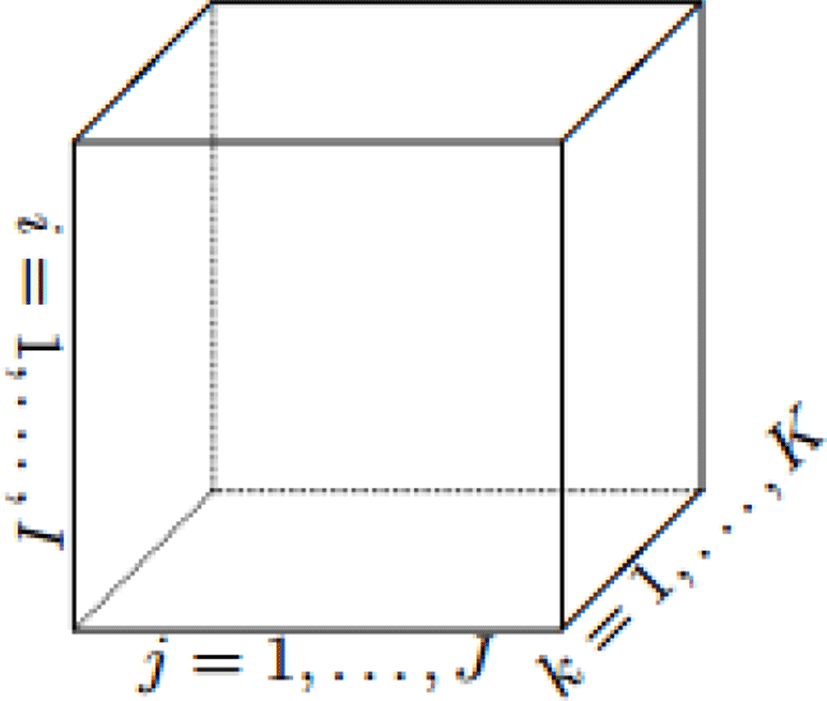
More clearly, a first-order tensor is a vector, a second-order tensor is a matric. Figure 2 represents a third-order tensor with three indices. The order of a tensor is the number of dimensions, also known as ways.
The definition of fibers in a tensor is for the higher order analogue of matrix rows and columns. When extracted from the tensor, fibers are always assumed to be oriented as column vectors.
Slices are two-dimensional sections of a tensor. A third-order tensor includes there slices: horizontal, lateral and frontal slices.
Matricization process of a tensor is the process of reordering the elements of an N-order tensor into a matrix.
Tensor elements (i1,i2,…,iN) maps to matrix element (in,j) where
Note that, the mode-n matricization of tensor 𝒳 is denoted by X(n) and arranges the mode-n fibers to be the columns of the outcome matrix.
The n-mode product of a tensor 𝒳 ∈ ℝI1×I2×…×IN with a matric U ∈ ℝJ×In denoted by 𝒳 ×nU and is of size
3.2. The Kronecker product I1 × … × In−1 × J × In+1 × … × IN. We note that, J will be replaced by the position of In for the n-mode product.
Elementwise, we have
Or we can rewrite as following:
III. THE TUCKER DECOMPOSITION
Tucker decomposition (TD) was firstly introduced by Tucker in 1963 and refined in 1966. The 1966’s version is the most comprehensive of the early literatures [4]. Tucker decomposition has many various names such as Higher-order SVD [5], N-mode SVD [6], three-mode factor analysis [7], N-mode principle components analysis [8].
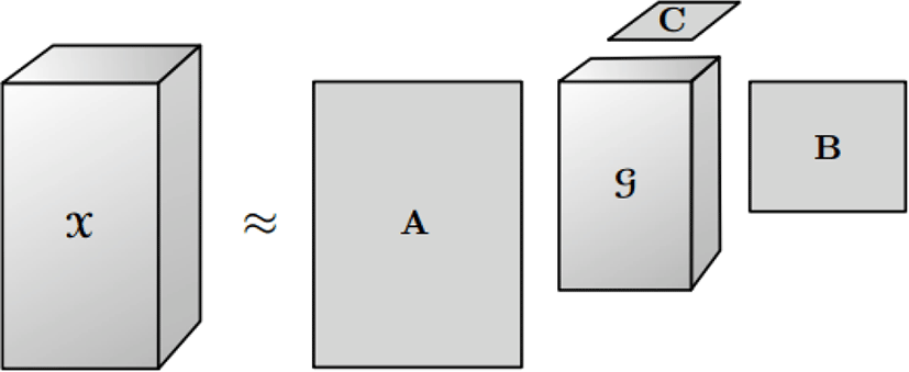
The Tucker decomposition is the form of higher order singular value decomposition. This method decomposes a tensor into a main part, called core, and some matrices alone each mode. Therefore, Tucker decomposition is indicated in the three-way case where 𝒳 ∈ ℝI×J×K as following:
Here, A ∈ ℝI×P, B ∈ ℝJ×Q, and C ∈ ℝK×R are the factor matrices and the tensor 𝒢 ∈ ℝP×Q×R is the core tensor after decomposing and its entries show the level of interaction between the different components.
Furthermore, P,Q and R are the number of components in factor matrices A,B,C, respectively. In some cases, the storage for the decomposed version of the tensor can be significantly smaller than for the original tensor. The Tucker decomposition is also illustrated in figure 3.
The metricized form of Tucker decomposition in the three-way case are
⊗ denotes the Kronecker product.
The Tucker model can be generalized to N-way tensors for third-order case as:
There are some methods to compute the Tucker decomposition. We also introduce one of them as in figure 5. It is called Tucker’s “Method I” introduced by Tucker in 1966.
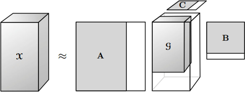
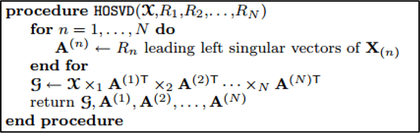
Figure 4 shows a truncated Tucker decomposition. The truncated TD is not optimal in terms of giving the best fit as measured by the norm of the difference. However, it is a good starting point for an iterative alternating least squares algorithm.
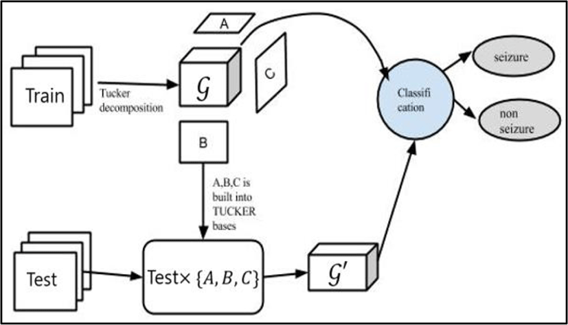
The data signals, in this paper, can be represented as a third-order tensor. Following [9], firstly, applying Tucker decomposition into the training set. After decomposing a three-way tensor data, we obtained another tensor 𝒢, called core tensor, and three matrices A,B,C.
Reduced features are obtained by projecting the data tensor onto the feature subspace spanned by basis factors A,B,C. In the other way, they are combined with the test part to build up the features for testing.
For more clearly, we consider a set (Train) of training samples and a set of test data (Test). The classification paradigm can be generally performed in these following steps:
-
Find the set of basis matrices and corresponding features for the training data.
-
Perform feature extraction for test data using the basis factor matrices found for the training data.
-
Perform classification by comparing the test features with the training features.
The core tensor represents that the feature is much lower dimension than the raw data tensor. In other words, the reduced core tensor consists of features of the training samples in the subspace of the factor matrices.
The conceptual diagram illustrating a classification procedure based on Tucker decomposition of all sampling training data is clearly represented in figure 6.
IV. NAÏVE BAYES FOR CLASSIFICATION
Naïve Bayes classification is a well-known probabilistic classifier and is widely used in the world. Naïve Bayes classifier is produced based on Bayes theorem with strong independence assumptions between the features as following:
Naive Bayes classifiers are highly scalable, requiring a number of parameters linear in the number of variables (features/predictors) in a learning problem. Naive Bayes is a simple technique for constructing classifiers: models that assign class labels to problem instances, represented as vectors of feature values.
Applying for the classification problem, with X =(x1,…,xn) represents the training data which was vectorized. Using Bayes’s theorem, the conditional probability can be decomposed as:
Where Ci is the ith possible outcomes or classes.
Therefore, we need to compute the probability of data over the outcome:
The algorithm of Naïve Bayes classifier can be summarized as following:
Step 1: Training Naïve Bayes based on the training data. Calculating P(Ci) and P(xk|Ci)
V. EXPERIMENT
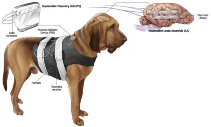
The EEG dataset was recorded from four dogs with naturally occurring epilepsy using an ambulatory monitoring system. The dogs were enrolled in the project by their owners, who were seeking better treatment options for their pets during routine veterinary care. This data set is gotten freely at the International Epilepsy Electrophysiology portal, developed by the University of Pennsylvania and the Mayo Clinic [11].
All of signals in this dataset are sampled at 400Hz with 16 electrodes spreading on each dog head.
Figure 7 shows the dog with its recording backpack. Two strips of 4 electrodes were placed on either side of the cortex and the data was recorded continuously for a prolonged period of time
The table 1 shows the number of segments in four dogs. The data used in this paper are arranged sequentially.
| Subjects | Dog 1 | Dog 2 | Dog 3 | Dog 4 |
|---|---|---|---|---|
| Non-seizure data | 418 | 1148 | 4760 | 2790 |
| Seizure data | 178 | 172 | 480 | 257 |
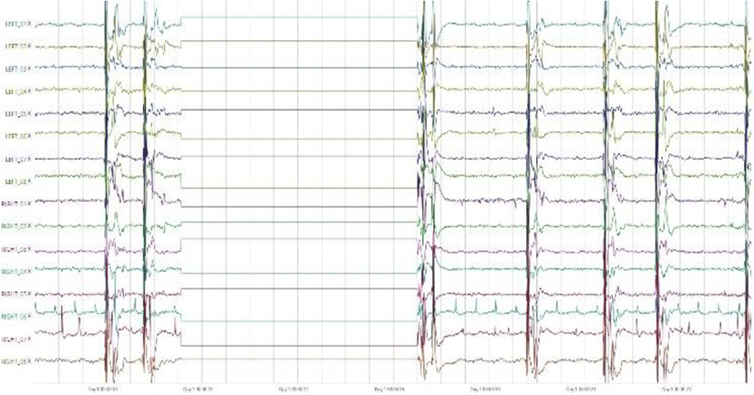
The figure 8 was plotted by the International Epilepsy Electrophysiology Portal’s tool with 16 electrodes in the first 30 seconds.
Dataset used in this paper is recorded to discriminate between seizure and non-seizure segments. Each segment is sampled in one second. The segments are arranged sequentially, firstly seizure segments, then non-seizure segments. The data will be rebuilt as a third-order tensor of size channels × time × segments to apply Tucker decomposition more easily.
The training data was constructed as a three-dimension tensor of size channels ×time × segments signals.
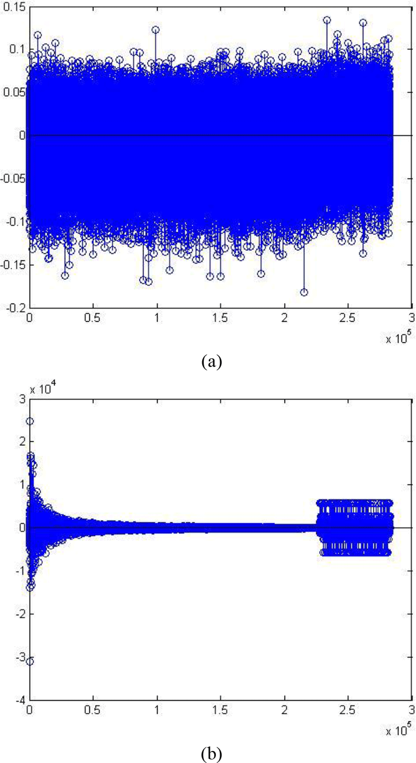
The comparison of original signal and decomposed signal is represented in figure 9. The original signal (a) still contains much noise. In figure 9(b), the seizure and non-seizure segments are clearly discriminated by plotting the signal in the core tensor. Because Tucker model extracts the good information in the raw data and only retains the best features of the signal. Therefore, the signal in figure 9(b) is very clear and contains quite little noise information.
To classify the data, we trained a Naïve Bayes classifier.
The accuracies of all dogs are always greater than 90 percent, even 95 percent. In the case, not using Tucker decomposition, the result of the first subject is quite bad, the accuracy is only approximately 79%. The other subjects get higher results, but not really good.
We also trained dataset using another classifier, Neural Network, but the obtained results are not good. Naïve Bayes using in this case is better. All results are showed in Table 2. We also know that Naïve Bayes is a very simple classification method. Many studies are shown that NB can work with a large number of attributes and similarly for classes. The accuracy of NB is calculated by the probability relationship of each data and each class. And in the case, the difference of classes is clearly discriminated, Naïve Bayes of course gives very good accuracies. About Neural Network, this is still a good classifier but theoretically, it needs to be retrained many times to get a good weight (not optimal weight) for each arc in the network. It is also dependent many decisions about hidden layers, topology and variants. We note that the accuracies are also affected by the dividing between the number of non-seizure and seizure samples in each subject as the case of Dog1.
| Subjects | Dog 1 | Dog 2 | Dog 3 | Dog 4 |
|---|---|---|---|---|
| Tucker + Naïve | 0.91 | 0.93 | 0.95 | 0.92 |
| Tucker + Neural | 0.62 | 0.84 | 0.61 | 0.69 |
| Non-Decomposition | 0.79 | 0.93 | 0.90 | 0.88 |
V. CONCLUSION
In this paper, a decomposition method is applied as a way to extract good features for EEG data in multidimensional space, specifically Tucker decomposition, or later known as Higher-order singular value decomposition (HOSVD).
The main goal of decomposition is “dividing” a multidimensional data into many parts which is smaller than original data but still contains full main information. A core tensor after decomposing a three-way data is a key feature for training. The remaining parts of this process will be contributed as the Tucker bases to build their test features.
Furthermore, the combination of Tucker decomposition and Naïve Bayes gave high accuracy. Naïve Bayes classifier is very useful and suitable for the case that has clear discrimination between two classes. Therefore, detecting a subject be a seizure or not becomes better.