Creation of 3D Maps for Satellite Communications to Support Ambulatory Rescue Operations

Nakajima, Isao; Nawaz, Muhammad Naeem; Juzoji, Hiroshi; Ta, Masuhisa

doi:10.33851/JMIS.2019.6.1.23

J Multimed Inf Syst 6(1):23-30

eISSN: 2383-7632

DOI: https://doi.org/10.33851/JMIS.2019.6.1.23

Section B

Creation of 3D Maps for Satellite Communications to Support Ambulatory Rescue Operations

Isao Nakajima¹^,^*, Muhammad Naeem Nawaz¹, Hiroshi Juzoji², Masuhisa Ta³

Author Information & Copyright ▼

¹Muhammad Naeem Nawaz, Tokai University, Isehara, Japan, mnaeemjapani@gmail.com

²Hiroshi Juzoji, EFL Inc. Takaoka, Japan., juzoji@yahoo.co.jp

³Masuhisa Ta, Tasada Works Ltd. Takaoka, Japan, tasada@lilac.ocn.ne.jp

^*Corresponding Author: Isao Nakajima, Tokai University, Isehara, Japan, js2hb@ets8.jp

© Copyright 2019 Korea Multimedia Society. This is an Open-Access article distributed under the terms of the Creative Commons Attribution Non-Commercial License (http://creativecommons.org/licenses/by-nc/4.0/) which permits unrestricted non-commercial use, distribution, and reproduction in any medium, provided the original work is properly cited.

Received: Mar 12, 2019 ; Revised: Mar 19, 2019 ; Accepted: Mar 21, 2019

Published Online: Mar 31, 2019

Abstract

A communications profile is a system that acquires information from communication links to an ambulance or other vehicle moving on a road and compiles a database based on this information. The equipment (six sets of HDTVs, fish-eye camera, satellite antenna with tracking system, and receiving power from the satellite beacon of the N-star) mounted on the roof of the vehicle, image data were obtained at Yokohama Japan. From these data, the polygon of the building was actually produced and has arranged on the map of the Geographical Survey Institute of a 50 m-mesh. The optical study (relationship between visibility rate and elevation angle) were performed on actual data taken by fish-eye lens, and simulated data by 3D-Map with polygons. There was no big difference. This 3D map system then predicts the communication links that will be available at a given location. For line-of-sight communication, optical analysis allows approximation if the frequency is sufficiently high. For non-line-of-sight communication, previously obtained electric power data can be used as reference information for approximation in certain cases when combined with predicted values calculated based on a 3D map. 3D maps are more effective than 2D maps for landing emergency medical helicopters on public roadways in the event of a disaster. Using advanced imaging technologies, we have produced a semi-automatic creation of a high-precision 3D map at Yokohama Yamashita Park and vicinity and assessed its effectiveness on telecommunications and ambulatory merits.

Keywords: Communications profile; Emergency patient transport; Polygon

I. PURPOSE

High-precision 3D maps based on advanced imaging technologies can be useful in establishing communication profiles for ambulance vehicles, visualizing transport routes (e.g., for landing emergency helicopters on public roadways or for rescues from high-rise buildings), and predicting tsunami damage. To assess the effectiveness of 3D maps for such applications, we produced a prototype 3D map of Yokohama Yamashita Park and vicinity. This paper presents an analysis and assessments of 3D maps and their applications in emergency medical services.

II. BACKGROUND

Polygon means the form where picture information was processed with the characteristic outline by computer graphics. Operation processing is reduced by this and a motion of a three-dimensional picture can respond in short time. The line concretely obtained from the outline of the building here is pointed out.

By the way, three-dimensional spatial data is the application to a car-navigation system such as Google Map(however -- fixing the viewpoint 1m in the height by the camera attached to the car) or widely used in various fields of guidance service. It is used for the space design of the simulation and environmental design of a townscape, a store, disaster refuge guidance, flood damage, a fire simulation, etc.

In a two-dimensional map, since the complicated geographic information of an unclear townscape can be visually grasped intelligibly with 3D(dimension) map, operators (include fireman, helicopter pilot) can understand a city atmosphere in the more nearly actually state.

At the manufacturing step of 3 map of a city area, it is from an aerial photograph.

There are many processes to create polygons from actual image, such as object removal of the outside for restoration, roadside tree for acquisition of building position information, the acquisition of height information using a laser range finder, and building appearance creation are included.

In this research, texture mapping of 3D polygon map was cut out from two or more continuous pictures from an in-vehicle camera with changing photography directions. It is able to create side part of the buildings from land mobile car. We can treat image distortion with geometric algorithm. Furthermore, the roof portion which cannot be taken from land mobile vehicle was created from image data from helicopter.

These two approaches (land and air) can make the building polygon by 3D.

Related these digital work, there are some paper reported to create building polygon automatically by graphic computers, however, under the present circumstances in a Japanese-styled house, it is very difficult to design and perform the full-automation of 3D polygon. Eventually, the building of each needs a check by human eyes.

III. METHODS

3.1. Mathematical Proof of Polygon

The principle which extracts points (points of Polygon) with the feature from an input picture [1-14], and its mathematical proof are as following. It is called the Scale Invariant Feature Transform: SIFT introduced by Dr. David G. Lowe who has the patent issue these formations [15].

3.1.1 Scale space

The gauss function G is defined as follows,

G (x, y, σ) = 1 2 π σ 2 e − (x 2 + y 2) / 2 σ 2

(1)

where I (x, y) is a function of an input picture and the function L (x, y) is defined,

L (x, y, σ) = G (x, y, σ) * I (x, y),

(2)

where D (x, y) which is a difference (Difference-of-Gaussian:DoG) of the smoothing picture which collapsed the input picture I (x, y) is defined from the following formula.

D (x, y, σ) = (G (x, y, k σ) − G (x, y, σ)) * I (x, y) = L (x, y, k σ) − L (x, y, σ) .

(3)

Consider the relationship of D(x,y) to σ²▽²G. The relationship between D(x,y) and σ²▽²G can be understood from the heat diffusion equation:

∂ G ∂ σ = σ ∇ 2 G

(4)

From this, we see V²G can be computed from the finite difference approximation to,

∂ G ∂ σ ≈ G (x, y, k σ) − G (x, y, σ) k σ − σ

(5)

and therefore

G (x, y, k σ) − G (x, y, σ) k σ − σ ≈ σ ∇ 2 G

(6)

G (x, y, k σ) − G (x, y, σ) ≈ (k − 1) σ 2 ∇ 2 G

(7)

When D(x,y) has scales differing by a constant factor it already incorporates the σ² scale normalization required for scale-invariance.

3.1.2 Localization

The 3D quadratic function is fit to the local sample points, and will start with Taylor expansion with sample point as the origin:

D (X) = D + ∂ D T ∂ X X+ 12 X T ∂ 2 D ∂ X 2 X,

(8)

where

X = (x, y, σ) T .

(9)

Take the derivative with respect to X, and set it to 0, giving

0 = ∂ D ∂ X + ∂ 2 D ∂ X 2 X^

(10)

the location of the keypoint

X^= − ∂ 2 D − 1 ∂ X 2 ∂ D ∂ X

(11)

This is a 3x3 linear system.as:

[∂ 2 D ∂ σ 2 ∂ 2 D ∂ σ y ∂ 2 D ∂ σ x ∂ 2 D ∂ σ y ∂ 2 D ∂ y 2 ∂ 2 D ∂ y x ∂ 2 D ∂ σ x ∂ 2 D ∂ y x ∂ 2 D ∂ x 2] [σ y x] = − [∂ D ∂ σ ∂ D ∂ y ∂ D ∂ x]

(12)

Derivatives approximated by finite differences, example:

∂ D ∂ σ = D k + 1 i, j − D k − 1 i, j 2 ∂ 2 D ∂ σ 2 = D k − 1 i, j − 2 D k i, j + D k + 1 i, j 1 ∂ 2 D ∂ σ y = (D k + 1 i + 1, j − D k − 1 i + 1, j) − (D k + 1 i − 1, j − D k − 1 i − 1, j) 4 .

(13)

If X is > 0.5 in any dimension, process repeated.

3.1.3. Filtering

Contrast can be described as:

D (X^) = D + 12 ∂ D T ∂ X X^.

(14)

If | D(X) | < 0.03, throw it out. To find Edgeiness, we use the ratio of principal curvatures to throw out poorly defined peaks.

Curvatures come from Hessian in the following:

H = [D x x D x y D x y D y y],

(15)

where Ratio of Trace(H)², sum of the diagonal components Tr(H), and Determinant(H)

If ratio > (r+1)²/(r), throw it out.

T r (H) = D x x + D y y D e t (H) = D x x + D y y − (D x y) 2

(16)

It can be understood as simple expressions:

T r (H) = α + β, D e t (H) = α ⋅ β .

(17)

3.1.4. Orientation assignment and descriptor

Based on these steps, descriptor computed relative to keypoint’s orientation achieves rotation invariance. Precomputed along for all levels and it is the most stable results, gradient magnitude: m(x,y) and orientation θ(x, y) is precomputed using pixel differences,

m (x, y) = (L (x + 1, y) − L (x − 1, y)) 2 + (L (x, y + 1) − L (x, y − 1)) 2 θ (x, y) = a tan 2 ((L (x, y + 1) − (L (x, y − 1) −)) / (L (x + 1, y) − L (x − 1, y))) .

(18)

The descriptor has three dimensions and multiple orientations has assigned to keypoints from an orientation histogram of gradient magnitudes.

3.2. Optical data collection

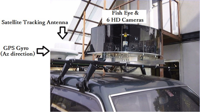
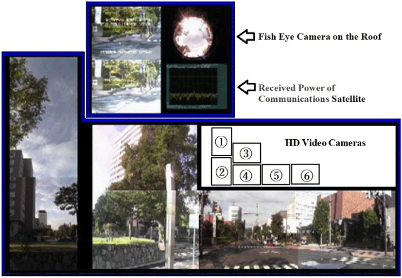
We used special vehicles, each mounted with a fish-eye camera lens facing straight up into the sky and as well as six high-definition cameras to obtain images of the surrounding area. We used this system to record images of the urban environment. The images and aerial photos obtained were used to produce a 3D map. Rather than placing the images of buildings and other structures on a simple flat map surface, we superimposed the images on a 50-m mesh elevation map published by the Geospatial Information Authority of Japan. Showing equally spaced grids to indicate area units of the same shape or size, mesh maps are generally used for quantitative analyses of various topographical information or to record a series of numerical data for each area unit. We used the vehicle's GPS positional data to obtain positional information corresponding to each image and obtained data on direction of travel from a GPS gyro. Our methods for producing the map information and converting location information to coordinates are based on the Numerical Map User’s Guide.1

Using these methods and software that was created by the authors, a 3D map of an area in Yokohama City was completed (Figure 1, 2). Still pictures of two or more sheets are continuously obtained from the moving vehicle (Figure 3). Each picture has spatial correlation and it becomes a spatial noise reduction by adding pictures.

Fig. 1. Area map.

Download Original Figure

Fig. 2. Aerial photo.

Download Original Figure

Fig. 3. Still picture of two or more sheets continuously are obtained from moving vehicle.

Download Original Figure

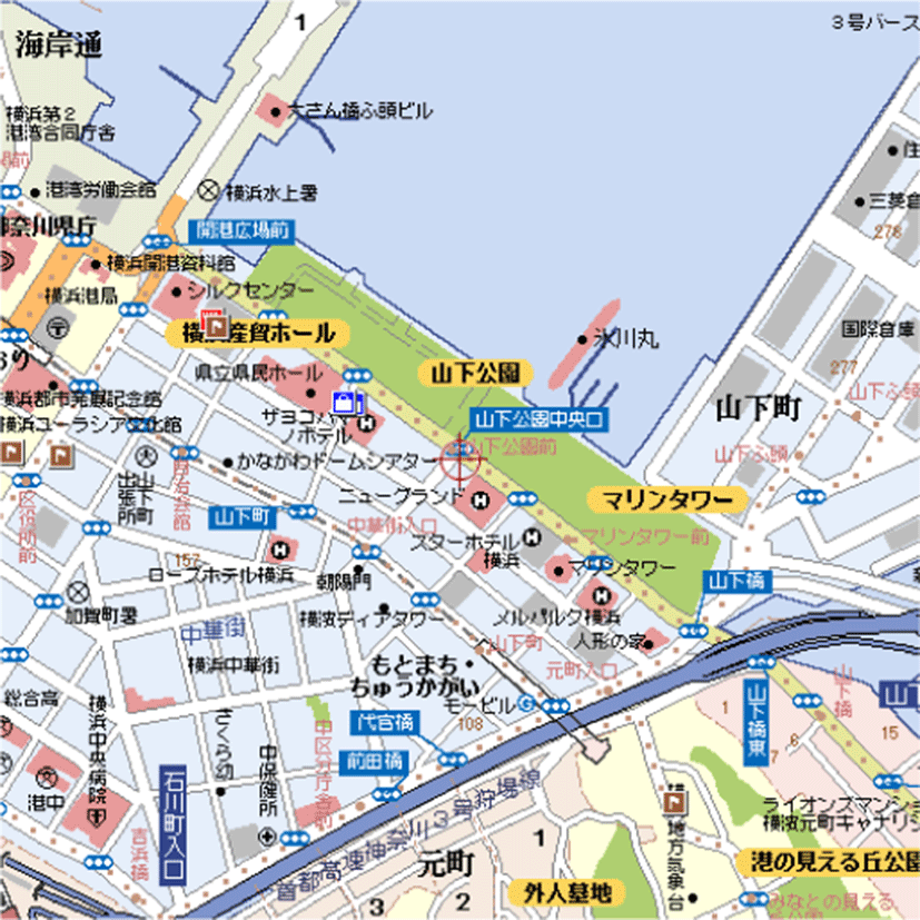
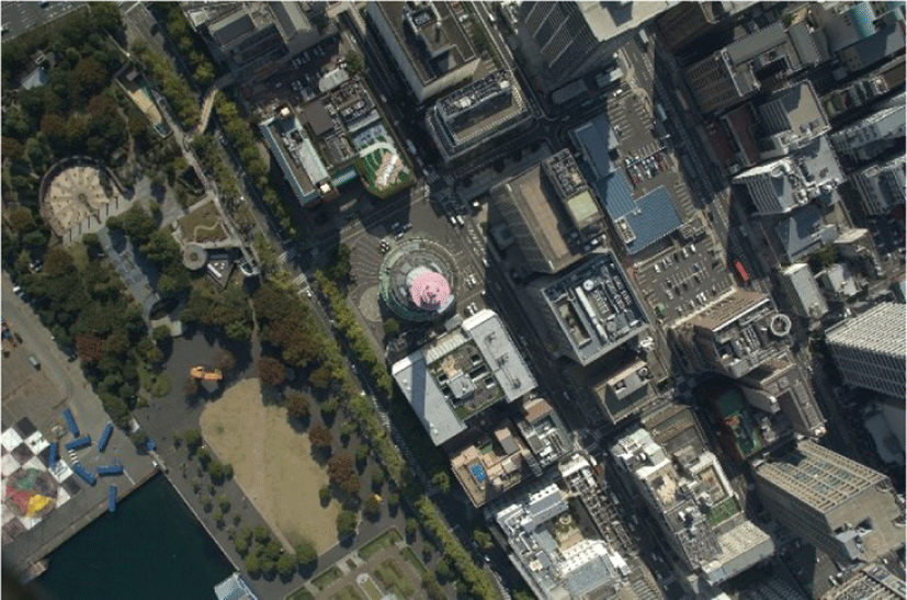
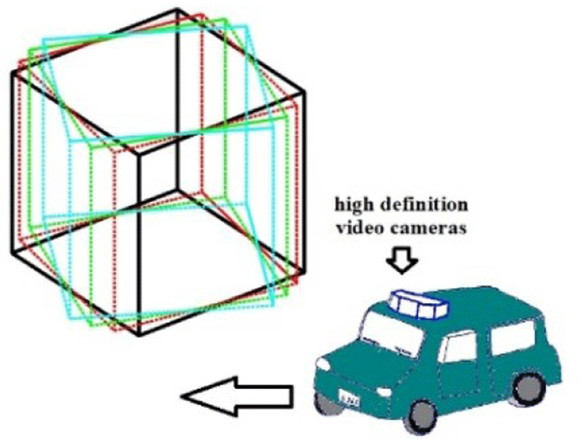
Figure 4 shows the mounted equipment on the roof of the vehicle, HDTV camera, GPS gyro and satellite tracking antenna, and Figure 5 displayed the motion pictures from each camera and NTSC image from spectrum analyzer. Every motion pictures were recorded by Panasonic HDCV video recorders. Table 1 lists the procedures for obtaining and processing images of an urban environment. For the purposes of our research, we prepared two special vehicles. Three dedicated staff members worked for two full years to acquire and process the images.

Fig. 4. Mounted equipment on the roof of the vehicle, HDTV camera, GPS gyro and satellite tracking antenna.

Download Original Figure

Fig. 5. Motion pictures from six sets of HDTVs and fish-eye camera carried on the roof of the vehicle and NTSC output from the spectrum analyzer showing the received signal of the satellite beacon.

Download Original Figure

Table 1. Procedures for acquiring and processing images.

	Procedures
1	Digital video recording with fish-eye lens and high-definition cameras from a moving vehicle
2	Calculating the height of building contours using images captured via fish-eye lens
3	Converting high-definition video images into AVI files to obtain still images
4	Producing still images of overhead views of buildings based on digital aerial photos
5	Placing optically distorted still images on polygons (contours) comprising each building
6	Placing polygons on a 50-m mesh elevation map published by the Geospatial Information Authority of Japan, which provides accurate height information
7	Embedding building information (e.g., addresses, tenants) as metadata
8	Adding information on underground structures (e.g., fire hydrants, sewer lines) as optional data

Download Excel Table

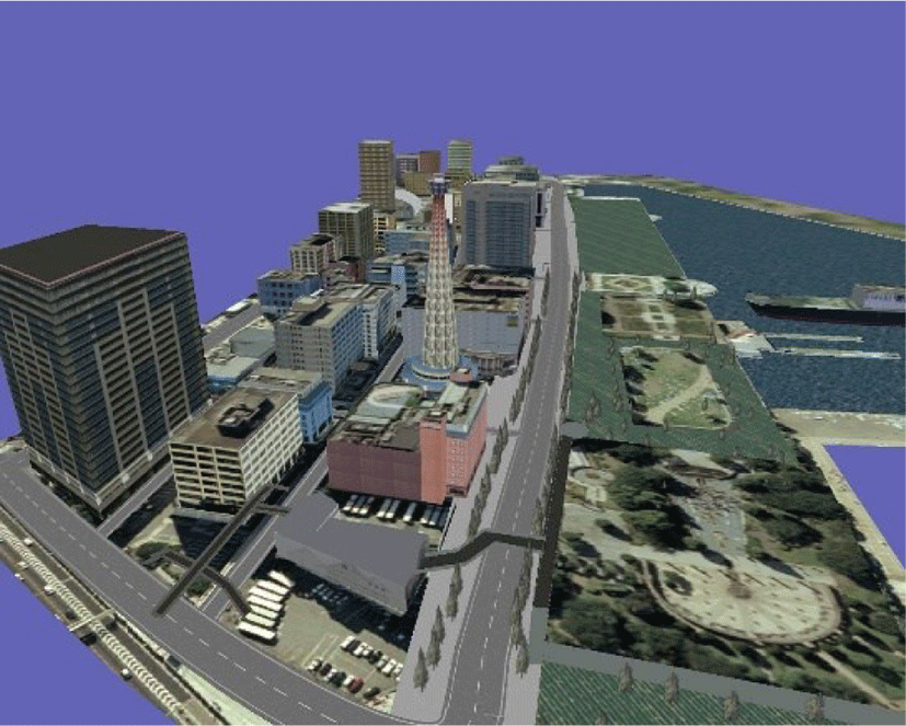
Finally, we can create the 3D map of the Yokohama Yamashita area with over 450 or more polygons. These polygons were put on 50m mesh map of the Geographical Survey Institute, and 3D map was completed. Figure 6 shows the resulting prototype of the 3D map of Yokohama Yamashita Park and its vicinity.

Fig. 6. Created 3D Map of Yokohama.

Download Original Figure

3.3. Mobile satellite signal

Geostationary satellite is the term for a communication/broadcasting satellite that remains at a certain orbital altitude above a specific point on the Earth at all times. They orbit in synchronization with the surface of the Earth at approximately 36,000 km above the equator. They are called geostationary because they appear fixed in the sky when viewed from the ground. One geostationary satellite can cover the whole nation. However, there is a major technological issue posed by the limited transmission power of a moving vehicle such as ambulance at urban area. This is the Blocking by buildings occurs because Japan is located at mid-latitude, not at the equator.

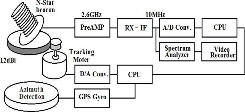
We have intended to monitor the beacon from N-Star of NTT DoCoMo on S-band. The block diagram is show in the Figure 7. This antenna system can track the satellite based on the GPS gyroscope (GPS gyro). The GPS gyro is made by Furuno Ltd. in order to provide Azimuth direction of moving vessel on the sea surface. It has three points antennas of GPS with 1m-triangle and has calculated the azimuth direction by having obtained the time lag(delay) of the GPS signals. Based on the azimuth data of the GPS gyro and the location data of the GPS, this tracking system can automatically beam 12dBi antenna to the satellite. Under the environment of line-of-sight propagation at the urban area, we can record microwave blockings generated between the vehicles and GEO satellite [16-18].

Fig. 7. Block diagram of the tracking system.

Download Original Figure

3.4. Comparison of actual optical blocking with fish-eye camera and simulation by polygons

With a fish-eye lens, the vehicle runs a comparatively large way in Yokohama, assumption direction of the satellite will be south (Az = 180 degrees), the actual optical relation of elevation angle were shown in Figure 8: Top. In actual blocking, the building form considered to be the first floor and the second floor is observed in a curve.

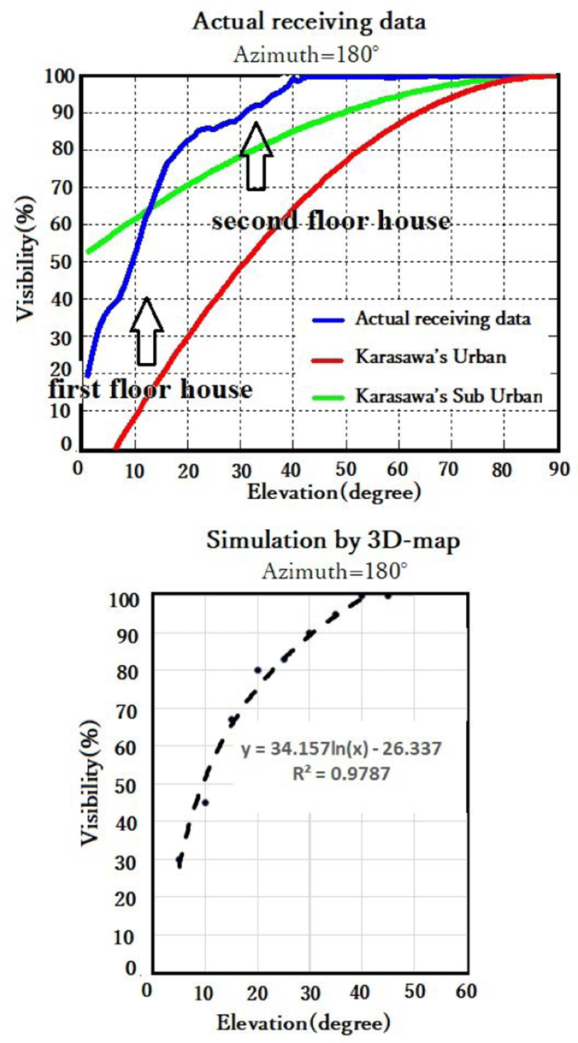
Fig. 8. Relationship between optical elevation angle and visibility (azimuth 180 degree) by fish-eye camera and by 3D map with polygons

Download Original Figure

Mr. Karasawa’s formula (approximate expression) of the elevation angle and visibility is provided in Table 2. The curve currently recorded has correlation in the curve of the Karasawa's sub urban formula comparatively. On the other hand, in 3D map created with polygons, the form difference of the building of the first floor and the second floor has disappeared (Figure 8: Bottom). It is because that polygons of buildings are expressed as a simple cube (matchbox) regardless of the portion which has pushed out to the road side of the first floor.

Table 2. Karasawa’s approximation by radio propagation.

Pa = 1 − a(90 − θ)²	θ > 10 degree
a = 1.43x10	Suburban
a = 6.0x10	Urban

Download Excel Table

IV. DISCUSSIONS

4.1 Discussion

4.1.1 Communication profile

During a disaster, there are two types of communication profiles recommended to perform smooth contact: ground wave communications and satellite communication. The propagation of line-of-sight is indispensable for the latter.

The latter will be predict beforehand with 3D-map with polygons. Based on this study, we can provide a satellite communications profile in Yokohama Yamashita area in future. However, the ground wave communications are synthesized by multipath waves reflected from buildings and artificial things. Composition of these reflective waves make frequency-selective fading channels, i.e., nonlinear propagation environment. On the other hand, assuming reflected waves of relatively high frequency (e.g., S band frequencies) from all directions, frequency-selective fading becomes flat fading. This allows relatively accurate predictions. On the spot, if received power could be recorded beforehand, the reliability of flat fading will be increased (not phase level but power level).

A communications profile is a system that acquires information from communications links to a moving ground vehicle and compiles a database based on this information. This system then predicts the communication links that will be available at a given location. For line-of-sight communication, optical analysis allows approximation if the frequency is sufficiently high. For non-line-of-sight communication, previously obtained electric power data can be used as reference information for approximations in certain cases when combined with predicted values calculated based on a 3D map.

In case of the terrestrial wave with elevation angle 10 degrees or less, it does not become real use. On the other hand, if the elevation angle for a satellite communication about 45 angles, 3D-Map made from the polygon may be able to predict communication as a communication profile.

4.1.2. Metadata

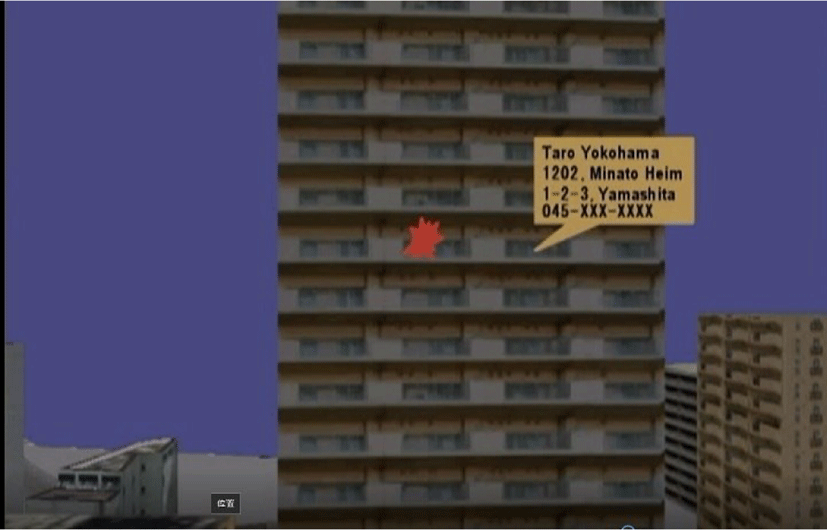
The planar map search devices currently used connect to a firefighting/emergency control board and automatically display a map of the target area when the location of the emergency caller or a landmark object is entered. It cannot render an image that depicts the environment more fully. In contrast, a 3D map shows a visually recognizable three-dimensional image of an emergency helicopter landing location or emergency transport route. A 3D map also allows predictions of areas likely to be affected by a tsunami immediately after an earthquake. Personal data, including telephone numbers, can be displayed on the map as metadata (Figure 9) to help facilitate communications and to help issue instructions for rescues from high-rise buildings.

Fig. 9. Metadata will be useful to confirm who he is at the building of the two or more floor.

Download Original Figure

4.1.3. On-road landing of emergency medical helicopters

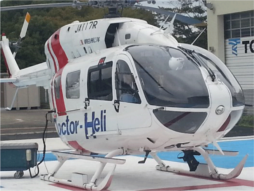
The first instance of an emergency medical helicopter landing on a road took place on March 10, 1972. An emergency medical helicopter was dispatched to the site of a head-on collision between a truck and a sightseeing bus on the Kanagawa Prefecture side of the Kobotoke Tunnel on the Chuo Expressway. The accident killed two and injured 41. The helicopter transported a physician from the Japan Ground Self-Defense Force Camp Ichigaya heliport. As part of rescue, emergency, and firefighting training for fires that might result from automobile accidents, on-road helicopter landing training was performed on August 2, 1985, before the Hanshin Expressway Route 7 Kita-Kobe expressway entered service. As part of this training, a helicopter landed near the Zenkai Interchange in Nishi Ward, Kobe City, for emergency patient transport. This training confirmed that a helicopter could land safely without the main rotor blades extending into oncoming traffic if it landed with its center positioned over the traffic median. In response to an accident on the Higashi-Kanto Expressway in the Kanto area in April 2002, an emergency medical helicopter on standby at the Nippon Medical School Chiba Hokusoh Hospital transported a physician to the accident site to treat the injured and then return with them to the hospital.

According to Aviation Law Enforcement Regulations of Japan revised in February 2000, if an emergency medical helicopter from a helicopter transport service company is dispatched to an emergency site in response to a request or notification by a firefighting or other such agency, takeoff and landing must proceed in the same way as with helicopters involved in search and rescue missions. This means emergency medical helicopters are permitted to land on public roadways in the event of emergencies. Landing a helicopter on a road requires an understanding of the three-dimensional positional relationships between nearby obstacles, including buildings and overhead power lines. Overhead power lines are clearly visible when an observer looks up into the sky; they are much more difficult to identify when an observer peers down against a background consisting of structures and the ground. Given the pressure to complete these missions as quickly as possible, it can be especially hazardous to make emergency landings immediately before rain or before sunset. All these circumstances make research on and the application of methods that provide support for on-road helicopter landings (and reduce risks in the event of emergency landings) quite valuable (Figure 10).

Fig. 10. Doctor Heli at Tokai university hospital.

Download Original Figure

4.1.4 Predicting tsunamis

Our 3D map is based on a 50-m mesh map published by the Geospatial Information Authority of Japan. The height information provided on this map is accurate, and we believe the map can be used to predict the range of areas affected in the event of a tsunami.

V. CONCLUSIONS

The equipment (six sets of HDTVs, fish-eye camera, satellite antenna with tracking system, and receiving power from the satellite beacon of the N star) mounted on the roof of the vehicle, image data were obtained at Yokohama Japan. From these data, the polygon of the building was actually produced and has arranged on the map of the Geographical Survey Institute of a 50 m mesh. The optical study (relationship between visibility rate and elevation angle) were performed on actual data taken by fish-eye lens, and simulated data by 3D map with polygons. There was no big difference. The 3D map system with polygons will be very useful to support ambulatory rescue operations during disaster.

Acknowledgement

The research described in this paper was carried out as a NEDO-subsidized project “Optical Analysis and Data Creation for Urban Environments, principal investigator: Isao Nakajima” We would like to show our greatest appreciation to Prof. Kiyoshi Kurokawa (ex-president of Medical Research laboratory, Tokai University, Isehara, Japan) for his appropriate guidance.

REFERENCES

[1].

T. Patterson, “Getting Real: Reflecting on the New Look of National Park Service Maps,” in Proceeding ofInt’l Cartographic Assoc. Mountain Cartography Workshop, 2002.

[2].

J.M. Airey, “Towards Image Realism with Interactive Update Rates in Complex Virtual Building Environments,” in Proc. 1990 Symp. Interactive 3D Graphics (SI3D 90), pp. 41-50, 1990.

[3].

D. CohenOr, “A Survey of Visibility for Walkthrough Applications” IEEE Trans. Visualization and Computer Graphics, Vol. 9, No. 3, pp. 412-431, 2003.

[4].

O. Sudarsky, C. Gotsman, “Output-Sensitive Rendering and Communication in Dynamic Virtual Environments,” in Proc. ACM Symp. Virtual Reality Software and Technology (VRST 97), pp. 217-223, 1997.

[5].

J.M. Zheng, R. Sundar, “Efficient terrain triangulation and modification algorithms for game applications,” in International Journal of Computer Games Technology - Joint International Conference on Cyber Games and Interactive Entertainment, Vol. 2008, Jan. 2006

[6].

Y. Livny, Z. Kogan, J. El-Sana, “Seamless patches for GPU-based terrain rendering,” The Visual Computer: International Journal of Computer Graphics, Vol. 25, No. 3, 2009, pp. 197-2008.

[7].

W.D. Pan, P. Yiannis, Y.F. He, “A vehicle-terrain system modeling and simulation approach to mobility analysis of vehicles on Soft Terrain” Proc. SPIE Unmanned Ground Vehicle Technology VI, Vol. 5422, pp. 520-531, 2004.

[8].

P.Maillot, “A new, fast method for 2D polygon clipping: analysis and software implementation,” ACM Transactions on Graphics (TOG), Vol. 11, No. 3, 1992, pp. 276-290.

[9].

F. Martinez, A.J. Rueda, F.R. Feito, “A new algorithm for computing Boolean operations on polygons,” Computers & Geosciences, Vol. 35, No. 6, 2009, pp. 1175-1185.

[10].

G. Bekker, Theory of Land Locomotion, University of Michigan Press, 1956.

[11].

D. Williams, “Volumetric representation of virtual environments,” Game Engine Gems, vol. 1, E. Lengyel, eds. Jones & Bartlett Publishers, 2010.

[12].

M. Rosa, Destructible volumetric terrain, GPU Pro: Advanced Rendering Techniques, W. Engel, eds., CRC Press, 2010.

[13].

Y. Zeng, C. Tan, W. Tai, M. Yang, C. Chiang ,C. Chang, “A momentum-based deformation system for granular material,” Computer Animation and Virtual Worlds, Vol. 18, issue (4-5), 2007, pp. 289-300.

[14].

Y. He, “Real-time visualization of dynamic terrain for ground vehicle simulation,” PhD Thesis, University of Iowa, 2000.

[15].

D. G. Lowe, “Distinctive Image Features from Scale-Invariant Keypoints” Int. J. of Computer Vision, vol.60, no.2, 2004, pp.91-110.

[16].

T. Kitano, H. Juzoji, I. Nakajima, “Elevation Angle of Quasi-Zenith Satellite to Exceed Limit of Satellite Visibility of Space Diversity which consisted of Two Geostationary Satellites”, IEEE Transactions on Aerospace and Electronic Systems, Vol. 48, No. 2, 2012, pp. 1779-1785.

[17].

T. Hatsuda, Y. Iwamori, M. Sasaki, Y. Tsushima, N. Yosimura, K. Kawasaki, T. Zakouji, M. Kuroda, K. Imai, Y. Maekawa, “Ku-band Time-Delayed Diversity/Satellite Diversity (TDD/Sat. D) system for improving link availability using lune-Q antenna”, in IEEE Antennas and Propagation Society International Symposium 2008, pp. 1-4, 2008.

[18].

Badan Nasional, Penanggulangan Bencana, “Peraturan Kepala BNPB No 02 Tahun 2012 tentang Pedoman Umum Pengkajian Risiko Bencana”, Jakarta, 2012.

[19].

Wirawan Prof, I.B. Su, “Pemetaan Daerah Rawan Konflik Sosial di Jawa Timur Dalam Rangka Ketahanan Nasional. Laporan Akhir Penelitian Unggulan Perguruan Tinggi Baru Tahap II”, Departemen Sosiologi Fakultas Ilmu Sosial dan Ilmu Politik University of Airlangga Surabaya, 2014.

[20].

Andi Ikmal Mahardy, “Analysis and Mapping of Flood Prone Areas in The City of Makassar Based On Spatial”, Departemen Teknik Sipil University of Hasanuddin Makassar, 2014.

[21].

Komang Sri Hartini, “Geographic Information System Applications of Public Works Infrastructure to Support Disaster Management (SIGI-PU),” Jakarta, 2013.

[22].

Riyanto, “Geographic Information System For Mapping disaster Prone Areas in Ponorogo,” Politeknik Elektronika Negeri Surabaya Surabaya, 2009.

[23].

Wikipedia. Indonesia, [online]: https://www.id.wikipedia.org/wiki/Indonesia.

[24].

Entin Martiana, “Logika Fuzzy”, Politeknik Elektronika Negeri Surabaya Surabaya.

[25].

“Undang-undang No 07 Tahun 2012 tentang Penanganan Konflik Sosial” in Presiden Republik Indonesia, Jakarta, 2012.

[26].

N. Ansari, B. Fong, Y. T. Zhang, “Wireless Technology Advances and Challenges for Telemedicine,” IEEE Communications Magazine, April 2006.

[27].

V. Patterson, J. Craig, R. Wootton, Introduction to Telemedicine, The Royal Society of Medicine Press, second Edition, 2006.

[28].

J. Craig, V. Patterson, “Introduction to the Practice of Telemedicine”, Journal of Telemedicine and Telecare, 2005.

[29].

V. Singh, “Telemedicine & Mobile Telemedicine System: An Overview”, 2000.

[30].

D. Ziadlou, A. Eslami, H. R. Hassam, “Telecommunication methods for implementation of telemedicine systems in crisis,” in Third International Conference on Broadband Communications, Information Technology & Biomedical Applications, 2008.

[31].

A. A. Aziz, R. Besar, “Application of Mobile Phone in Medical Image Transmission,” in Fourth National Conference on Telecommunication Technology Proceedings, 2003.

[32].

J.J. Perez-Sevilla, D.C. McLernon, “Medical image transmission over a GSM cellular system”, Electronics Letters, Vol. 36, No.16, August 2000.

[33].

Wireless Telemedicine System in Emergency Medicine Helicopter. Available from: https://www.researchgate.net/publication/228905726_Wireless_Telemedicine_System_in_Emergency_Medicine_Helicopter [accessed Mar 07 2019].

[34].

C. S. Pattichis, E. Kyriacou, S. Voskarides, M.S. Pattichis, R. lstepanian, C. N. Schizas, ”Wireless Telemedicine Systems: An Overview”, IEEE Antenna’s and Propagation Magazine, Vol. 44, No. 2, April 2002.

[35].

S. Voskarides, C. S. Pattichis, R. Istepanian, E. Kyriacou, M. S. Pattichis, C. N. Schizas, ”Mobile health systems: A brief overview”, Healthcom 2002, Vol.1, pp.50-56, June 2002.

[36].

A. Shokrollahi, LDPC Codes: An Introduction, April 2, 2003.

[37].

A. F. Molisch, “Wireless Communications,” IEEE Press, 2005.

[38].

K. Thenmozhi, V.Prithiviraj, “Suitability of Coded Orthogonal Frequency Division Multiplexing (COFDM) for Multimedia data transmission in Wireless Telemedicine Applications,” in International Conference on Computational Intelligence and Multimedia Applications, 2007.