I. INTRODUCTION
Single image super resolution (SISR) is a classical computer vision task to reconstruct a high-resolution (HR) image from a low-resolution image. SISR is used for various applications such as surveillance imaging [1], medical imaging [2] and, HDTV in recent years. In order to improve accuracy in the restored image, there have been a lot of efforts, such as SRCNN [3], VDSR [4], and EDSR [5] which use deep learning that is a breakthrough in image restoration.
Solutions to more accurate image restoration had previously been thought to require deeper networks, with techniques such as deep residual learning [6] and batch normalization [7], which unfortunately lead to a huge sum of parameters. Several other state-of-the-art methods emphasize the importance of architectural structure for better performance, but still require heavy computation. On the other hand, studies for practical operation and high efficiency aim to reduce computation whilst maintaining accuracy. However, studies on multi-scalability have not been enough. Multi-scalability refers to multiple scale image restoration by using a single model, which is essential in practical applications.
Methods implementing pre-up-sampling techniques like SRCNN [3], VDSR [4], DRCN [8] involve an interpolation- based up-sampling method (bicubic interpolation). Networks up-sampling with bicubic interpolation can be trained to restore images by multiple scale factors via a single model. VDSR [4] showed better performance by using a single model trained on multiple scales compared to the performance by using different models for each scale. Scale augmentation can also be considered as data augmentation, thus yielding generalization of the model. Techniques which are also multi-scaled and involve multi-path learning ex. MDSR [5] prove the existence of shared parameters across different restoring scale factors.
Studies show that pre-up-sampling techniques induce a significant number of operations compared to post-up-sampling SR frameworks. In this paper, we introduce an efficient multi-scalable convolutional neural network constituting post-up-sampling but interpolation-based upscale technique. Similar to BTSRN [9], the proposed network consists of convolutional layers applied on the low-resolution input image and its feature maps, an up-sampling layer, and more convolutional layers applied on the up-scaled feature maps. Unlike BTSRN [9], in the upscale layer, the multiple-channeled feature map of the previous layer is up-scaled by bicubic interpolation inducing multi-scalability. Additionally, unlike other previous works of which the training is performed using only scale factors of 2, 3, and 4, the proposed network is trained by using real-number scale factors in the range of 1.5 to 4.0.
II. RELATED WORKS
The implementation of convolutional neural networks to execute computer vision tasks such as image classification and image generation has been very successful. We can solve classification tasks, for example, identifying diseases in plants [10], and even group images based on its pixel contents for effective image retrieval from large databases, just as implemented in [11]. Image generation tasks like document binarization [12] are more advanced, and adversarial networks can be implemented. Super resolution falls into the category of image generation, as the output is also an image, but with a higher resolution.
Image restoration can be achieved in several ways, but the applied upscaling method is an essential factor. Traditional upscale methods include nearest-neighboring, bilinear and bicubic interpolation, which are interpolation techniques applied on a 2-Dimensional matrix. Amongst them, bicubic interpolation has the best performance, and it has been applied in various software applications for image upscale. Its efficiency lies in the ability to enlarge a given image to any ratio and scale.
Architectural frameworks like SRCNN [3] show an implementation of bicubic interpolation on low-resolution (LR) images as a preprocessing measure to enlarge them. The images are then refined by the convolutional neural network to produce an output with better quality measured in PSNR. SRCNN [3] was a breakthrough in the area of super resolution due to its deep learning application with the implementation of LR-HR non-linear mapping. However, it proposed a shallow network consisting of only 3-layer and also concluded the impossibility of a deeper network. VDSR [4] on the other hand, was able to implement a deep convolutional network with the application of a residual framework improving output image quality. Further studies such as DRCN [8], DRRN [13] & MemNet [14] on frame-work structure were also made for better performance.
Depending on framework structure, upscaling methods have significant effect on the performance, the number of operations, and the number of learning weights (parameters). FSRCNN [15] and ESPCN [16] do not use interpolation-based upscale. Instead, learning based up-sampling methods (transposed convolution [17] and sub-pixel shuffling [16]) were used, in which up-sampling was implemented at the last layer of the network (which is post-up-sampling), indicating implementation of convolution in the LR space only. This breakthrough improved performance and reduced the number of operations (multi-adds) significantly. It efficiently improved image restoration techniques in general, making them more accurate and faster. SRResNet [18], EDSR [5], SRGAN [18], and other works involving post-up-sampling techniques (mostly sub-pixel shuffle and transposed convolution) have been able to produce state-of-the-art performances in super-resolution. However, these methods require large computing operations and large number of parameters which are impractical. Although performances are outstanding in comparison, they might not be worth it in most application environments, and are thus, not efficient.
Fast, accurate, and efficient approaches such as CARN [19], FALSR [20], BTSRN [9] were made to cope with real-time applications. These have shown possibilities to reduce computations and parameters significantly while maintaining moderate performance, making implementation possible in most environments. Nevertheless, frameworks with transposed convolution or sub-pixel shuffling can train only a single model per a single upscale factor. Therefore, separate models have to be trained to restore images to different scales implying the inability of multi-scalability via a single model.
Looking into earlier SR techniques, VDSR [4] did not only show better performance in comparison to its previous works, but it also introduced multi-scalability via a single model. In previous works, networks are trained separately for upscale factors of 2, 3, and 4. However, VDSR [4] introduced a single model capable of training and testing on different scales. This was possible due to its reliance on the interpolation-based up-sampling technique. At any cost, studies show that pre-up-sampling-based frameworks lead to significantly huge computations and do not perform well compared to post-up-sampling-based SR methods.
More recent studies like MDSR [5] claim to have made a breakthrough on single model multi-scalability by introducing scale multi-path learning. In structures of scale multi-path learning models, there are three output ends for the three (×2, ×3, and ×4) upscale factors, as a result, being able to produce SR outputs of different scales. The first few layers of this architecture have shared parameters proving similarities across different scales. On the downside, practical applications do not involve only fixed number (integers) scale factors. In most practical applications, output images eventually have to implement an interpolation-based technique to produce desired output image size. This would require the need to train a single model involving real-number upscale factors which was unfortunately, even not implemented in VDSR [4] during training. Additionally, when upscaling LR images to a certain HR size, the other ends of the network will be useless taking up memory space. In this paper, we introduce an efficient SR technique, able to output images of any desired size. We utilize the post-up-sampling method for efficient practical operations.
III. PROPOSED METHOD
The CNN deep residual network learns to a non-linear mapping between the ground-truth (high-resolution images) and its low-resolution counterpart.
The identity image is the upscaled LR image via bicubic interpolation, and the network learns its residual for the reconstructed SR result. Therefore, the dataset consists of the LR image, its bicubic upscaled image, and the HR ground-truth image. The residual image, r, is given by:
where B represents the bicubic operation, x is the LR image, and y is the ground truth. The loss function is defined as the mean squared error (MSE) of the residual and the predicted output of the LR image input:
where n represents the number of training samples, m is the number of image data per a single training sample. F refers to the operation of the network performed on the x input data to produce the predicted output.
The architecture of the proposed method is a two-staged residual network. As expressed in Figure 1, Convolutional layers and ReLU activation layers are for feature extraction, bicubic interpolation is then used for up-sampling, and additional layers are applied for SR image reconstruction. Inspired by VDSR [4], we up-sample the identity image via bicubic interpolation, and add it to the residual output making it a residual network. In the convolutional neural network (CNN), the kernel size and number of filters are 3 × 3 and 64 respectively. ReLU is used as its activation function. In the LR stage, the residual network is deployed with 8 blocks while 2 more blocks are deployed at the HR stage after up-sampling. This network consists of 10 residual blocks in total.
We perform up-sampling with bicubic interpolation on all channels of the extracted feature map on the last layer of the LR stage as shown in Figure 1. Interpolation-based (bicubic) pre-up-sampling SR methods [21] have always been used on the LR image, which is only 1(grayscale) channeled. Up-sampling in this case is applied on channels of extracted feature (64 channels). The up-sampling layer is located not at the very end but a few layers before the last. Therefore, this can be called a post-up-sampling network.
Restored images are able to possess any possible size and ratio utilizing interpolation-based up-sampling tech-niques due to their nature of referencing surrounding pixels for the upscaled image reconstruction. Super resolution in previous works has not been able to emphasize real-number upscale factors. In practical application, upscale factors to enlarge images are not always fixed. For example, upscaling an HD+ display (1024 × 768) size to fit a 4K UHD (3840 × 2160) display while maintaining the same aspect ratio is impossible with a fixed upscale factor of 2. Its upscale factor is 2.4. The image will have to upscale by a factor of 2, thereby depending on the remaining 0.4 to be upscaled by an interpolation-based technique. Conclusively, interpolation-based up-sampling techniques are essential in almost all applications. Corres-pondingly, we learn a mapping between LR and HR image datasets, not only with fixed scale factors but also with real-number upscale factors within the range of 1.5 to 4.0. Compared to previous works training on only 3 different upscale factors (×2, ×3, and ×4), we train with 11 different scales for better accuracy in all circumstances. The performance also improves as the complexity in real-number training scale factors increases. We train our model on the limited number of upscaling factors, but inference implementation can be done to output any size and ratio.
Compared to a pre-up-sampling network like VDSR [4], computation is reduced and performance is better. In comparison with the VDSR [4] model, the Number of parameters, multi-adds, and other properties is as shown in Table 1. More computation is executed in bicubic interpolation compared to bilinear and nearest-neighboring. Figure 1 shows that 64 channeled feature-maps are being up-scaled via bicubic interpolation. Hence, we also calculate and add the number of operations executed by the upscaling layer to the multi-adds column in Table 1. We use the bicubic polynomial equation to calculate the multi-add operations of the up-sampling layer, just as done in [18]. According to the bicubic polynomial equation, to fill up every missing pixel after spreading pixels apart (for upscaling), 9 multi-adds operation has to be executed per missing pixel.
| Properties | Proposed | VDSR [4] |
|---|---|---|
| Training scales | 1.5, 1.75, 2, 2.25, 2.5, 2.75, 3, 3.25, 3.5, 3.75, 4 | 2, 3, 4 |
| Parameters | 296K | 665K |
| Multi-adds | 49.9G | 612.6G |
| Number of layers | 10 | 20 |
The architecture consists of three main factors - feature extraction, up-sampling, and image reconstruction. Residual blocks in the LR stage learn a set of 64 channeled feature map to be up-sampled via bicubic interpolation as shown in Figure 1. It plays the most important role in this framework, hence consists of 8 layers. Feature-maps in the up-sampling layers are the results of the analyzed LR image, creating the best format to up-sample via bicubic interpolation. After feature map up-sampling, the HR stage has 2 residual layers for HR image reconstruction.
IV. EXPERIMENTS AND RESULTS
The performance of the proposed method is evaluated, and it is compared with the performance of the VDSR [4], and other multi-scale networks. For all experiments excluding benchmarking, we utilize the 291 images in [4].
For training, we crop images in the dataset to make the LR sub-images (image patches) the size of 20 × 20. The network is trained with 11 different scales increasing by 0.25 from 1.5 to 4.0, which means that the sizes of HR sub-images are 30, 35, 40, 45, 50, 55, 60, 65, 70, 75, and 80, respectively. Because sub-image sizes cannot be represented in float types, the LR sub-image size is carefully chosen to put the receptive-field concept into account. The LR sub-image size and the 0.25 step size of scale are determined in order to make the corresponding HR sub-image sizes integer figures. Data augmentations included: flip, rotation, and downsizing, with dataset increasing due to scale number complexity. Cropped HR image patch was downscaled via bicubic interpolation to create x (LR) dataset. LR and HR sub-images in each batch have to be of the same size, hence each batch represented an upscale factor, and training iteration was performed on a randomly assigned batch.
We train the models with adaptive momentum optimizer [22] and 128 mini-batch sizes. Training is done over 275,000 iterations with an initial learning rate of 10-3 exponentially decaying to 10-5. Iterations are roughly the same (a little over 275,000) for all performed experiments. Maintaining iteration number, more epochs (to repeat iterations of the same set of data) are needed for training on the deeper networks due to the reduced amount of dataset. Deeper networks have larger receptive fields, hence require larger sub-image sizes. Xavier normal [23] is used to initialize weights before training. All implementations are executed utilizing the PyTorch [24] deep learning tool and training lasts for roughly 5 hours on RTX 2080.
After image cropping, the size of the HR sub-images ranges from 30 up to 80. In VDSR [4], the dataset was created downsizing by all required scales, upscaling via bicubic and cropping. All cropped sub-images are combined forming a larger dataset. In the proposed method, however, cropping images for a single network is a tricky task, because the number of all datasets have to be equal across all scales for equality during training. Data augmentation techniques with the priority being – original image, left-right flipping, rotation by 90°, 180°, 270°, and downsizing are used to solve this problem. First, we crop the dataset images to sub-images for the largest HR sub-image size needed (80 × 80). The amount of the cropped HR sub-images is then used as the limit value to stop creating more sub-images (by cropping) when reached by other HR sub-image sizes. Hence, not all augmentation techniques will be utilized as scale factor decreases.
Set 5 [26], Set14 [27], BSD 100 [28] and Urban 100 [30] datasets are used for testing and comparing results with previous works. The datasets, especially Set 5 [26] with different scale factors are used to evaluate the performance of different structures and strategies of the proposed method.
It was mentioned in Section 3 that the LR stage and HR stage represent feature extraction and image reconstruction respectively. However, to reduce the computational com-plexity of the network, experiments are made to reduce the number of residual blocks on the HR stage while increasing those of the LR stage. This experiment is also done in comparison with VDSR [4].
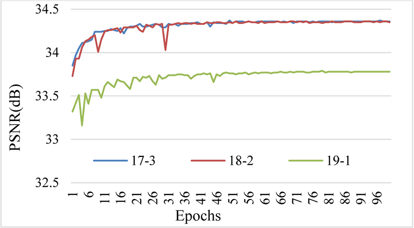
For a fair comparison, training is done with 20 layers and with the upscaling factor of 2, 3, and 4. The number of the LR and HR stages residual blocks lead to difference in performance, showing the importance of the up-sample layer’s location. To maintain the number of residual blocks in the network, the increased feature extracting layers (layers in LR stage) means reducing HR image reconstructing layers. As shown in Table 2, when LR-HR blocks are 17 - 3 and 18 - 2, the difference in performance measured in PSNR is less than 0.01 which is negligible.
| Proposed PSNR (dB) and SSIM results | VDSR [4] | |||
|---|---|---|---|---|
| Scale LR-HR |
17 - 3 PSNR / SSIM |
18 - 2 PSNR / SSIM |
19 - 1 PSNR / SSIM |
0 - 20 PSNR / SSIM |
| × 2 | 37.5733 / 0.9588 | 37.5659 / 0.9588 | 37.0928 / 0.9513 | 37.53 / 0.9587 |
| × 3 | 33.9024 / 0.9232 | 33.8976 / 0.9229 | 33.3120 / 0.9072 | 33.66 / 0.9213 |
| × 4 | 31.5304 / 0.8865 | 31.5334 / 0.8859 | 30.8687 / 0.8622 | 31.35 / 0.8838 |
| Average | 34.34 / 0.9228 | 34.33 / 0.9225 | 33.76 / 0.9069 | 34.18 / 0.9213 |
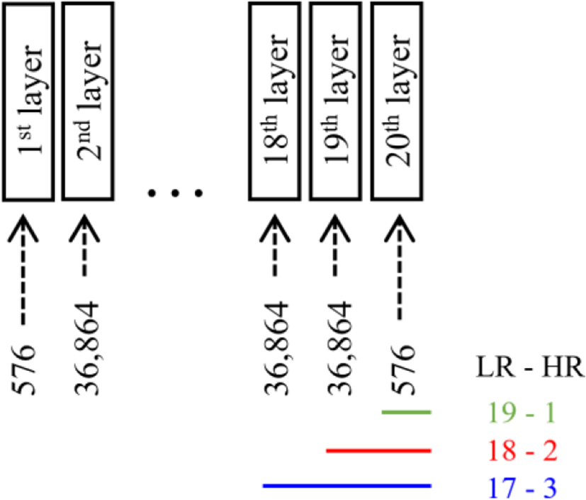
19 - 1 LR-HR blocks display reduction in performance due to excessive reduction in the number of parameters as shown in Figure 2. 19-1 implies 19 LR blocks and just 1 layer on the HR space, which is the last layer of the network (the first and last layers of SR networks usually possess the least number of parameters). The difference in parameter numbers in the HR stages between 17-3, 18-2, and 19-1 are 74,304, 37,440, and 576 (each hidden layer has 36,864 parameters) respectively. 576 parameters are too small for image reconstruction regardless of having more in the LR stage, therefore 37,440 parameters in the HR stage (18-2 LR-HR blocks) were concluded as the best for a trade-off between performance and efficiency of the network. Compared to VDSR [4], this (20 layers 18-2) network reduces the computation significantly. The training process can be observed in Figure 3, and there is little to no difference in performance between 17-3 and 18-2.
For more efficient results, we reduce the number of residual blocks to 10 layers. The previous experiment emphasizes the need for 2 layers in the HR stage, which denotes that reduction should be done in the LR stage layers if required. Reduction from 18-2 (20 layers) to 8-2 (10 layers) LR-HR stages are experimented and results were similar as shown in Table 3. The difference of the overall average on the testing datasets is approximately 0.1 (in PSNR), which is trivial. Although the VDSR [4] model is successfully trained on the 291 [29], [30] images dataset, its receptive field was not large (due to pre-up-sampling) compared to the proposed method, hence sub-images had to be cropped to a large size, making 291 [29], [30] images dataset insufficient on the proposed 20 layers (18-2) network. The 10 layers network had a similar performance while the amount of computation is reduced by 29.8% compared to the 18-2 LR-HR layers, and by 91.9% compared to VDSR [4], when we assume the HR image resolution is 720P and the upscaling factor is ×4.
| Dataset | Scale\LR-HR | 18 - 2 PSNR/SSIM | 8 - 2 PSNR/SSIM | VDSR [4] PSNR/SSIM |
|---|---|---|---|---|
| Set 5 | × 2 | 37.57/0.9588 | 37.52/0.9585 | 37.53/0.9587 |
| × 3 | 33.90/0.9229 | 33.85/0.9226 | 33.66/0.9213 | |
| × 4 | 31.53/0.8859 | 31.48/0.8854 | 31.35/0.8838 | |
| × 2 | 33.01/0.9139 | 33.01/0.9137 | 33.03/0.9124 | |
| Set 14 | × 3 | 29.87/0.8367 | 29.86/0.8364 | 29.77/0.8314 |
| × 4 | 28.26/0.7787 | 28.26/0.7782 | 28.01/0.7674 | |
| × 2 | 31.91/0.8959 | 31.89/0.8954 | 31.90/0.8960 | |
| B100 | × 3 | 28.85/0.7985 | 28.84/0.7981 | 28.82/0.7976 |
| × 4 | 28.34/0.7266 | 27.33/0.7262 | 27.29/0.7251 | |
| Urban 100 | × 2 | 30.77/0.9146 | 30.73/0.9138 | 30.76/0.9140 |
| × 3 | 27.14/0.8289 | 27.14/0.8286 | 27.14/0.8279 | |
| × 4 | 25.25/0.7554 | 25.26/0.7553 | 25.18/0.7524 | |
| Average | 30.53/0.8514 | 30.43/0.8510 | 30.37/0.8490 | |
| Parameters | 665K | 296K | 665K | |
| Multi-adds | 71.1G | 49.9G | 612.6G | |
All results in Tables 2 and 3 are based on experiments done by training with only 2, 3, and 4 upscale factors for fair comparison and accurate evaluation. In reality, however, image restoration to up-sample images to any size should be possible. Table 4 shows results based on training the 10 layers network by more complex upscaling factors. The model was additionally trained by upscaling factors in the range of 1.5 to 4.0 with a step of 0.5 (1.5, 2, 2.5, 3, 3.5, 4), and also with a step of 0.25 (1.5, 1.75, 2, 2.25, 2.5, 2.75, 3, 3.25, 3.5, 3.75, 4). The difference is between 3, 6, and 11 upscaling factor values. Greater numbers of upscaling factor values give more complexity to the model. The results of VDSR [4] with real-number upscaling factors are obtained by using the official model in [31]. VDSR [4] results have poor performance especially on 1.5 and 1.75 scales, possibly due to its nature of pre-upscaling.
| Dataset | Testing scale\Trained scales | 2, 3, 4 PSNR/SSIM | 1.5, 2, 2.5, 3, 2.5, 4 PSNR/SSIM | 1.5, 1.75, 2, 2.25, 2.5, 2.75, 3, 3.25, 3.5, 3.75, 4 PSNR/SSIM | VDSR [4, 28] (2, 3, 4) PSNR/SSIM |
|---|---|---|---|---|---|
| Set 5 | 1.5 | 40.40/0.9766 | 40.62/0.9771 | 40.59/0.9770 | 33.54/0.9503 |
| 1.75 | 38.81/0.9677 | 38.81/0.9677 | 38.82/0.9677 | 35.91/0.9572 | |
| 2 | 37.52/0.9585 | 37.49/0.9584 | 37.49/0.9585 | 37.53/0.9587 | |
| 2.25 | 36.40/0.9496 | 36.34/0.9495 | 36.37/0.9495 | 35.12/0.9416 | |
| 2.5 | 35.39/0.9404 | 35.41/0.9406 | 35.45/0.9406 | 34.34/0.9325 | |
| 2.75 | 34.66/0.9326 | 34.63/0.9327 | 34.68/0.9328 | 33.54/0.9265 | |
| 3 | 33.85/0.9226 | 33.83/0.9226 | 33.86/0.9228 | 33.66/0.9213 | |
| 3.25 | 33.18/0.9137 | 33.13/0.9137 | 33.20/0.9138 | 32.47/0.9080 | |
| 3.5 | 32.64/0.9042 | 32.66/0.9045 | 32.69/0.9046 | 32.18/0.9006 | |
| 3.75 | 32.00/0.8957 | 31.99/0.8955 | 31.98/0.8953 | 31.57/0.8914 | |
| 4 | 31.48/0.8854 | 31.51/0.8852 | 31.50/0.8853 | 31.34/0.8838 |
Results are tested with Set 5 [26] and with the 11 scaling factors. The results in Table 4 lead to a conclusion that scale complexity improves performance. More scale augmentation creates more batches for training which is essential. Theoretically, reconstructed (SR) images would have more quality on real-number upscale compared to models that are trained with only 2, 3, and 4 upscale factors.
All the previous experiments are done by training using the addition of T91 [29] and BSD200 [30] image datasets just as performed in VDSR [4]. We use the addition of T91 [29], BSDS 200 [30] and General 100 [32] to train the model for benchmarking results on Table 5 and Figure 4.
| Scale | Model | Params | Multi-Adds | Set 5 PSNR/SSIM | Set 14 PSNR/SSIM | B 100 PSNR/SSIM | Urban 100 PSNR/SSIM | Real-number Upscale |
|---|---|---|---|---|---|---|---|---|
| 2 | VDSR [4] | 665K | 612.6G | 37.53/0.9587 | 33.03/0.9124 | 31.90/0.8960 | 30.76/0.9140 | No |
| LapSRN [34] | 813K | 29.9G | 37.52/0.9590 | 33.08/0.9130 | 31.80/0.8950 | 30.41/0.9100 | No | |
| MPRNet [31] | 538K | - | 38.08/0.9608 | 33.79/0.9196 | 32.25/0.9004 | 32.52/0.9317 | No | |
| EMSR (ours) | 296K | 94.5G | 37.57/0.9588 | 33.16/0.9144 | 31.95/0.8959 | 30.99/0.9162 | Yes | |
| 3 | VDSR [4] | 665K | 612.6G | 33.66/0.9213 | 29.77/0.8314 | 28.82/0.7976 | 27.14/0.8279 | No |
| MPRNet [31] | 538K | - | 34.57/0.9285 | 30.42/0.8441 | 29.17/0.8073 | 28.42/0.8578 | No | |
| EMSR (ours) | 296K | 61.4G | 33.92/0.9235 | 29.91/0.8370 | 28.89/0.7980 | 27.31/0.8324 | Yes | |
| VDSR [4] | 665K | 612.6G | 31.35/0.8838 | 28.01/0.7674 | 27.29/0.7251 | 25.18/0.7524 | No | |
| 4 | LapSRN [34] | 813K | 149.4G | 31.54/0.8850 | 28.19/0.7720 | 27.32/0.7280 | 25.21/0.7560 | No |
| MPRNet [31] | 538K | 31.3G | 32.38/0.8969 | 28.69/0.7841 | 27.63/0.7385 | 26.31/0.7921 | No | |
| EMSR (ours) | 296K | 49.9G | 31.59/0.8863 | 28.33/0.7797 | 27.36/0.7267 | 25.38/0.7590 | Yes |
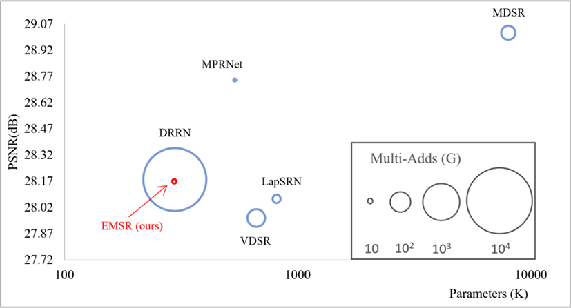
Two main key elements in this paper are real-number multi-scalability and efficiency in practical implementation. Models such as CARN [19], FALSR [20], BTSR [9], and OISR [33] are state-of-the-art methods excelling in efficiency while maintaining impressive levels of performance. Nevertheless, they do not have the ability to restore images with multiple upscaling factors, thus needing multiple trained models for implementation on several upscale factors, which we can arguably be referred to as inefficient. Therefore, the comparison was done with state-of-the-art methods that can perform multi-scale learning using a single model.
The comparison is performed with VDSR [4], LapSRN [33], MDSR [5], DRRN [13] and MPRNet [35]. Results in Figure 4 are based on scale factor ×4 to show superiority in post-up-sampling techniques. The results prove efficiency in parameters and operation numbers while maintaining good performance.
The proposed model is also able to perform real-number upscaling. The results in Table 5 leaves out MDSR [5] and DRRN [13] due to their bulkiness in computation and parameters. MPRNet [35] provides good results with less computation, but Table 5 show that more parameters are used compared to the proposed model.
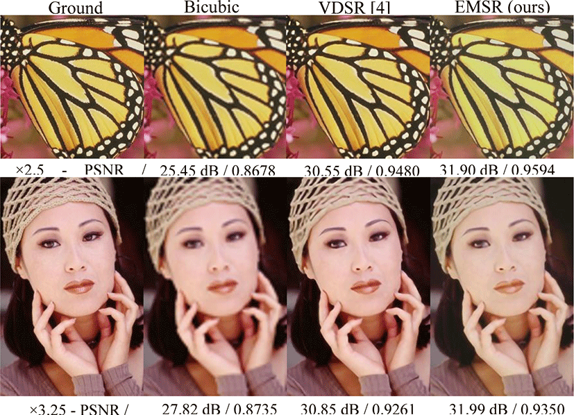
Figure 5 shows visual comparison with VDSR [4]. Major differences cannot be seen visually, but the results in PSNR indicate improvement in performance.
V. CONCLUSION
The proposed (EMSR) model is able to find a break-through in interpolation-based post-up-sampling with a more realistic and efficient outcome.
Using a single model for vast complexity with a small number of parameters and less computation pushes its ability to the limit without waste. Our model can generate images to any possible size and ratio well within the range of trained upscale while maintaining a very reasonable amount of quality. Further works can be done on the architectural structure for even better performance whilst maintaining its efficiency.


