I. INTRODUCTION
As multimedia technology advances, new types of video formats such as ultra-high-definition (UHD), virtual reality (VR), and 360-degree video has emerged. Accordingly, the needs of novel video coding standard that can support higher resolution videos and better coding efficiency are increasing. Versatile Video Coding (VVC) was developed by the Joint Video Exploration Team (JVET), a collaboration between VCEG and MPEG [1]. It was finalized in July 2020. As the latest video coding standard, the VVC adopts several new coding schemes and tools, such as coding tree unit (CTU) with a maximum size of 128×128, quad-tree plus multi-type tree (QT+MTT) structure of coding unit (CU) partition and affine motion compensation prediction. These new techniques achieve about 50% gain over the HEVC standard in terms of bit rate reduction. However, the computational complexity of both encoding and decoding has also increased sharply.
n [2], the time complexity of VVC Test Model (VTM) was analyzed compared to HEVC Test Model (HM). Figure 1 compares the normalized total average complexity of the HEVC and VVC encoder with all 720p and 1080p test sequences [3]. The VVC encoder takes 5, 7, and 31 times as much time as the encoding time of the HEVC under Low Delay (LD), Random Access (RA), and All Intra (AI) configurations, respectively.
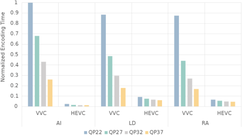
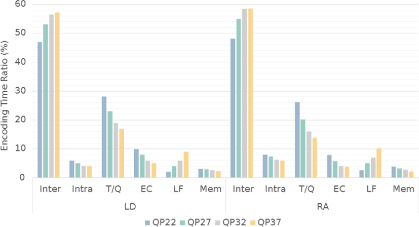
In Figure 2, the complexity breakdown of the VVC encoder is presented. The total complexity is broken down into six categories of Inter-prediction (Inter), Intra prediction (Intra), Transform and Quantization (T/Q), Entropy Coding (EC), Loop Filters (LF), and Memory (Mem) operations. Out of all the encoding tools, inter-coding accounts for the highest portion of the total encoding time in LD and RA. In addition, the QT+MTT structure causes much more recursive calls to coding tool functions than that of the quad-tree structure of the HEVC.
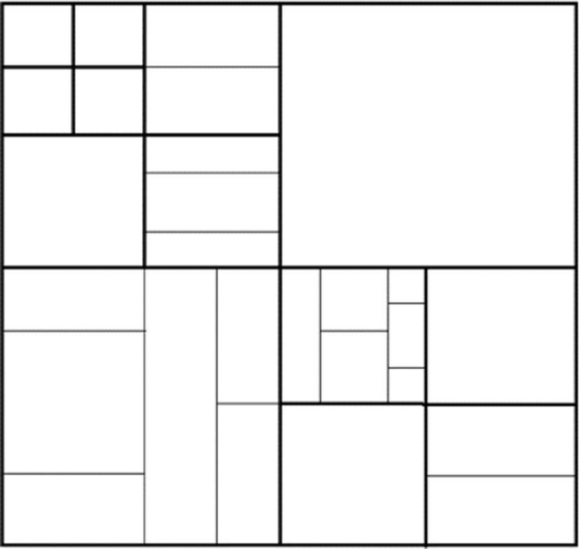
A new approach is needed for the complexity optimization for the VVC inter-coding and the QT+MTT partitioning. With QT+MTT partitioning structure, a CU can be split among quad-tree (QT), binary-tree (BT), ternary-tree (TT). Also, horizontal (H) and vertical (V) direction split can be applied in BT and TT. Therefore, total of 6 split modes (Non-split, QT, BT_H, BT_V, TT_H, TT_V) are available for a CU. Figure 3 shows the possible split modes, and the Figure 4 represents an example of CTU that is partitioned by the QT+MTT structure. To be more specific, a CTU is first partitioned by the QT structure. Then, the QT leaf nodes that are CUs can be further partitioned by the QT or MTT structure.
For the inter prediction, the VVC encoder takes advantage of the redundancy that exists between pictures (inter pictures). After partitioned into blocks, motion compensation is applied for each block. Inter prediction mode has mainly two coding methods: Advanced motion vector prediction (AMVP) mode and Merge mode. In AMVP mode, the optimal values of multiple motion vector candidates, the motion vector difference value, the reference picture number, and the uni-/bi-directional prediction mode are encoded. In merge mode, only the optimal value of multiple motion vector candidates is encoded. The AMVP mode has the advantage of freely determining and coding parameters, while the number of bits required for coding the parameter is high, and requires a complex coding process, motion estimation. For the Merge mode, the number of bits required for coding is very small, but the prediction value is inaccurate.
In this study, we define the problem as deciding a split mode for a coding tree unit (CTU) by using a convolutional neural network (CNN).
We propose a CNN architecture called multi-level tree CNN (MLT-CNN). The MLT-CNN is used during the encoding process and is implemented in VVC Test Model (VTM) 11.0. In addition, some additional information including inter-picture information is used to boost the training performance of CNN.
The remainder of this paper is divided as follows: In Section 2, we give a summarization of the related works in HEVC and VVC. In Section 3, we first observe which information can be useful to train the MLT-CNN model, present the MLT-CNN architecture, and then outline the overall algorithm. The experimental results are shown in Section 4. Lastly, the paper closes with a conclusion and a preview of future work in Section 5.
II. RELATED WORKS
Kim et al. proposed an inter mode decision algorithm based on temporal correlation in H.264/AVC [5]. In [6], the RD cost distribution and spatial correlation were jointly adopted for fast CU mode decision in HEVC intra coding. Lim et al. utilized the RD cost as the key feature to skip PU early and terminate early based on Bayes decision rule [7]. In [8], an early skip detection method for HEVC was proposed based on the identification of motionless and regions with homogeneous texture in a video sequence. A fast inter-mode decision algorithm for HEVC was proposed by exploiting both the spatio-temporal correlations and the inter CU correlation of quad-tree structure among neighboring CUs, in which the prediction mode, MV, and RD cost were found strongly correlated [9].
Zhang et al. proposed a scheme based on the relationship between impossible modes and distribution of distortion to accelerate the inter coding in HEVC [10]. Xiong et al. proposed a fast inter CU decision algorithm for HEVC based on the latent sum of absolute difference (SAD) estimation by defining the concepts of two-layer motion estimation and motion compensation RD cost [11]. Lee et al. proposed a PU decision algorithm based on correlation and block motion complexity (BMC) for HEVC [12]. Goswami et al. utilized a Bayesian classifier for skip detection and coding unit termination in HEVC [13].
The advantages of these algorithms are simple, easy to implement, and hardware friendly. Also, they are usually efficient due to the limited complexity overhead. However, these approaches have some limits: Only a small number of critical features can be exploited in each algorithm, and the thresholds of these algorithms are usually determined based on the statistical analyses on a small set.
For the deep learning-based approach, Jin et al. used a convolutional neural network (CNN) to predict the range of CU depth in each 32×32 CU, skipping the rate-distortion optimization (RDO) search of unused CUs at intra-mode [14]. Another CNN-based approach is to predict CU depth range at inter-prediction mode, which uses a residual CU as the CNN input since the partition relies on the correlation between the current frame and the reference frames [15]. Considering that various CU partition results may satisfy the same depth range, the models in [14], [15] can hardly predict the exact CU partition. Thus, they are limited in reducing the complexity of the VVC.
Subsequently, Galpin et al. [16] suggested a scheme deciding the CU partition directly by predicting all possible CU boundaries between adjacent 4×4 blocks using ResNet model [17]. But the bottom-up decision causes unnecessary calculation when a CTU is non-split or split into only a few large CUs in Kim et al. adopted CNN to predict split or non-split for CU depth decision both inter and intra-coding in the HEVC [18]. Lee et al. have improved visual quality for HEVC using CNN [19]. They constructed a little simple network model for intra prediction mode. In [20], a CNN based fast CU mode decision algorithm is devised for HEVC inter-prediction. The CNN takes the features of the integer motion estimation (IME) and then determines the partition modes in advance. Li et al. proposed a method for VVC intra-coding, where multiple CNNs are trained for various CU sizes to decide whether the CU should be split by which kind of partitioning [21].
Some studies for VVC intra-coding have been done; however, few studies yet consider the characteristics of inter-prediction. As some studies show, CNN based approach is suitable for dealing with images. The most recent work proposed in [15] takes quad-tree plus binary-tree (QTBT) structure. Also, this method predicts each coding unit (CU) depth, therefore it needs more RDO process.
As far as we know, no previous research has studied complexity reduction for inter-prediction within QT+MTT structure using CNN. Thus, we propose a fast split mode decision method that handles with QT+MTT structure by utilizing a CNN to decide CU split type efficiently in the inter-coding process. In this paper, a new CNN architecture that fits QT+MTT structure of the VVC to predict the split mode of each square CU is proposed. In addition, we present a fast decision algorithm using additional temporal information to reduce time complexity for inter-coding in the VVC encoder.
III. PROPOSED METHOD
In this section, observation and analysis are made on block shapes for various conditions to design a CNN architecture suited to QT+MTT structure.
Figure 5 shows an equivalent frame encoded with all intra (AI) and random access (RA) configuration (picture order count (POC)=1, BasketballDrive from VVC test sequences). This represents split tendency difference between intra-picture prediction (intra prediction) and inter-picture prediction (inter prediction). Each block is split finely when encoded with all intra prediction than when encoded with inter prediction mode. During the intra prediction process, a prediction block is constructed using neighboring pixels, and a residual block is obtained by subtracting the original block and the prediction block pixel by pixel. Meanwhile, the prediction block is found by referencing other pictures during the inter-mode prediction process. Therefore, it is not enough to characterize a split mode of a CU with only original CU image in the inter prediction. Furthermore, this leads to why we should make use of the residual image as well as the original image of CU for CNN based inter mode CU partitioning decision.
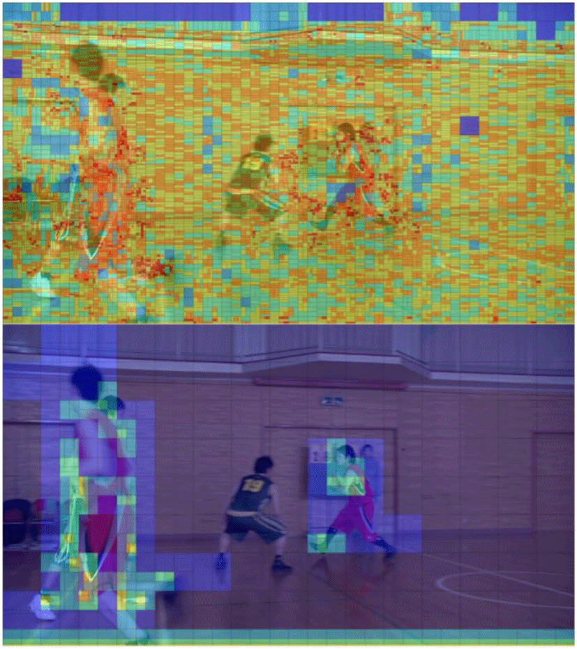
In this work, we target square-shaped CUs as CNN input. Specifically, 128×128 blocks are used for training. In addition, since square-shaped CU which is split by QT can be further split by QT or MTT, it has more cases to be split. This means that QT leaf node, e.g., square-shaped CU, has more opportunity to reduce time compared to other shapes through early termination.
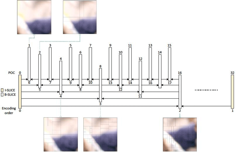
As shown in Figure 6 and Figure 7, split types are different from quantization parameter (QP) value and POC value. In Figure 6, there shows CTUs in (0, 0) position in BasketballDrive sequence encoded with each of five QPs (22, 27, 32, 37, and 42). The QP reflects the compression of spatial details. If QP is large, some details are lost and the image quality is reduced. Therefore, the larger the QP value for the same block is, the shallower the split depth is. Additionally, Figure 6 illustrates CTU in (128, 0) position in Tango2 sequence with different POC under QP=22 and RA configuration. One can notice that the CTU with a deeper temporal layer tends to be split further. As shown in Figure 7, the first picture in group of pictures (GOP) is encoded as intra picture and all the other pictures within the GOP are encoded as B or GPB pictures. Encoding order in the first GOP is as follows: the picture with POC 8 refers POC 0, and then the picture with POC 4 is encoded referring POC 0 and 8. As such, the temporal layer gets deeper according to the referred pictures.
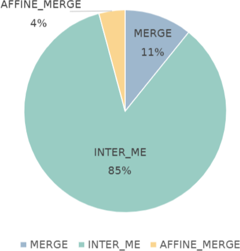
Figure 8 shows the encoding time ratio of three inter prediction modes (Affine MERGE, MERGE, and Inter ME mode) for all CTUs. Encoding time was measured with Campfire sequence from CTC sequences with QP={22, 27, 32, 37, 42}. It shows that two merge modes take much less time than that of the Inter ME process. Therefore, it is entirely reasonable to predict the split mode of CU using a CNN after performing merge modes to decide whether to skip Inter ME and split directly. In this stage, the residual image is obtained from the current best CU for training CNN.
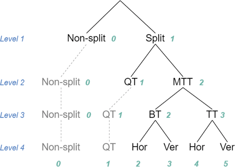
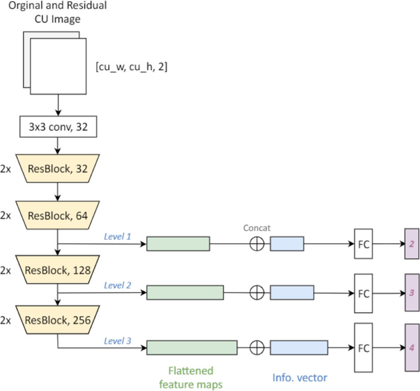
In this study, we propose a multi-level tree CNN (MLT-CNN) architecture that fits QT+MTT structure of the VVC standard. The architecture is modified from Branch-CNN (B-CNN) [22]. The B-CNN is suitable for training labels with a hierarchical structure because it predicts labels in a coarse-to-fine manner. The major difference between MLT-CNN and the B-CNN is that the additional feature vector is used in each level to improve training performance and we use the residual block [23] as a basic block. The MLT-CNN network predicts a split mode among four split modes for CUs with 128×128, since the ternary-tree split is restricted for CTU level. The key feature of the network is that it predicts split mode per each level similar to the split mode tree structure described in Figure 9.
The equation of the cross entropy loss is denoted by:
where yi and ŷl are the ground-truth and the predicted score for each class i, and C is the number of classes. Also, ŷı is calculated by:
The weighted categorical cross-entropy loss is used for training the MLT-CNN:
where L denotes the number of levels in CNN. The weight Wl changes by iteration so that the loss of each level can be reflected effectively. In this experiment, Wl changes every 150k iterations; Wl=[0.97, 0.02, 0.01] for 0-150k, [0.97, 0.02, 0.01] for 150k-300k, [0.1, 0.1, 0.8] for 300k-450k, and [0, 0, 1] for the last 150k iterations. By setting weights different from iteration, CNN can learn the characteristics of the hierarchical split mode tree. In the early stages of training, the CNN model learns the labels of level 1 (split or non-split) by giving more weights on the loss of level 1. As learning progresses, more weight is given to the lower level. It helps to solve complex problem more effectively than learning from scratch.
Figure 10 shows the architecture of the MLT-CNN. The network consists of four ResBlocks with three levels. First, the 128×128 original and residual image which can be obtained after performing MERGE modes are concatenated as a CNN input. Then, 3×3 kernels at the first convolutional layer is used to extract the low-level features. Before each level prediction, feature maps are further convoluted with residual blocks (ResBlocks).
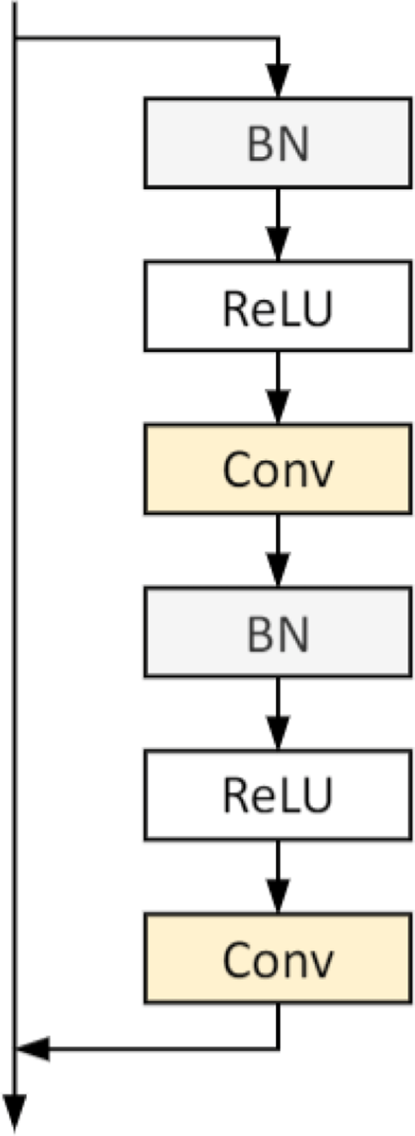
The detail of ResBlock is depicted in Figure 11. For each level, feature maps are flattened and concatenated with information vector which includes POC, and the CU-level QP. If each of them is not available, it is zeroed. These additional data help improve the performance of training. Finally, the concatenated tensor goes through one fully connected (FC) layer. The effects of using additional information will be shown in Section 4.
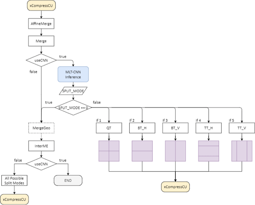
The overall process of the proposed algorithm using the MLT-CNN is shown in Figure 12. The VVC test model, VTM-11.0, was used as the baseline and additional implementation was carried out. After performing MERGE mode in the encoding process, the inference is performed using original, residual image, and POC, and the CU QP.
If the predicted split mode is 0 (Non-split), then it keeps performing other modes such as inter motion estimation and intra prediction, and then no further split occurs. If the predicted split mode is bigger than 0, it means CU needs to be directly split and no other split mode for the current depth is performed. Split modes 1, 2, 3, 4, and 5 represent QT, BT_H, BT_V, TT_H, and TT_V respectively.
IV. EXPERIMENTS AND DISCUSSION
A training database for deep video compression called BVI-DVC [24] is used in this paper. All sequences in the BVI-DVC are progressive-scanned at a spatial resolution of 3840×2160, with frame rates ranging from 24 fps to 120 fps, a bit depth of 10 bit, and in YUV420 format. Also, each sequence has total of 64 frames. There are 200 kinds of video clips and they are augmented with 3 resolutions: 1920×1080, 960×540, 480×270. Therefore, the resulting number of sequences is 800 with four different resolutions.
We classified all the sequences into three groups according to the motion degree of each video. Among the whole sequences, 23 kinds of sequences were selected: 9, 7, and 7 sequences in the order of high motion degree. 20 sequences used for training CNN are AmericanFootballS3Harmonics, BasketballGoalScoredS2Videvo, BricksTiltingBVITexture, BuildingRoofS3IRIS, CharactersYonseiUniversity, ColourfulRugsMoroccoVidevo, FerrisWheelTurningVidevo, FireS18Mitch, HamsterBVIHFR, HongKongMarket4S1Videvo, LakeYonseiUniversity, ManStandinginProduceTruckVidevo, MoroccanCeramicsShopVidevo, MuralPaintingVievo, PillowsTransBVITexture, RunnersSJTU, SquareS1IRIS, StreetDancerS3IRIS, TraditionalIndonesianKecakVidevo, and WatPhoTempleVidevo, and 3 sequences for validating CNN during training are CostaRicaS3Harmonics, FireS21Mitch, and ResidentialBuildingSJTU. Each kind of sequence can have four different resolutions, so 92 sequences were used for building the dataset.
In VVC Test Model (VTM) 11.0 encoder, the residual image is acquired right after Merge mode as the best CU at that point under the Random Access (RA) configuration. The other information such as picture order count (POC), and CU-level QP value are obtained from the decoding process. Table 1 shows the number of train and validation data of 128×128 size.
| 128×128 | NON | QT | BT_H | BT_V | Total |
|---|---|---|---|---|---|
| Train | 1,136,495 | 521,929 | 115,699 | 129,277 | 1,903,400 |
| Validation | 6,702 | 14,364 | 1,387 | 1,847 | 24,300 |
| total | 1,143,197 | 536,293 | 117,086 | 131,124 | 1,927,700 |
All models were trained using the PyTorch deep learning framework [25] with a single GPU for training. Table 2 shows the specifications of the experimental environment. In all experiments, we use Adam optimizer [26] with α1=0.9, α2=0.99; initial learning rate 0.0004 that decays with the cosine annealing schedule [27]. To assess the training performance, the validation accuracy over the validation dataset was measured.
| OS | Ubuntu 16.04 |
| CPU | Intel Xeon Processor (Skylake, IBRS) (2.6GHz) |
| GPU | NVIDIA Tesla V100 (32GB) |
| Mem | 103GB |
To prove the performance with using additional information including temporal features such as residual image and POC helps improve training performance, we compare the validation accuracy between the ResNet trained only with the original CU images (ResNet_O), ResNet trained with the original and residual images (ResNet_OR), and ResNet trained with the original, residual images and the information vector (ResNet_ORI). As shown in Figure 13 and Figure 14, the ResNet_ORI shows the highest validation accuracy, and the ResNet_OR shows higher validation accuracy and lower training loss than those of ResNet_O.
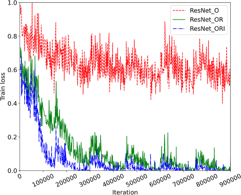
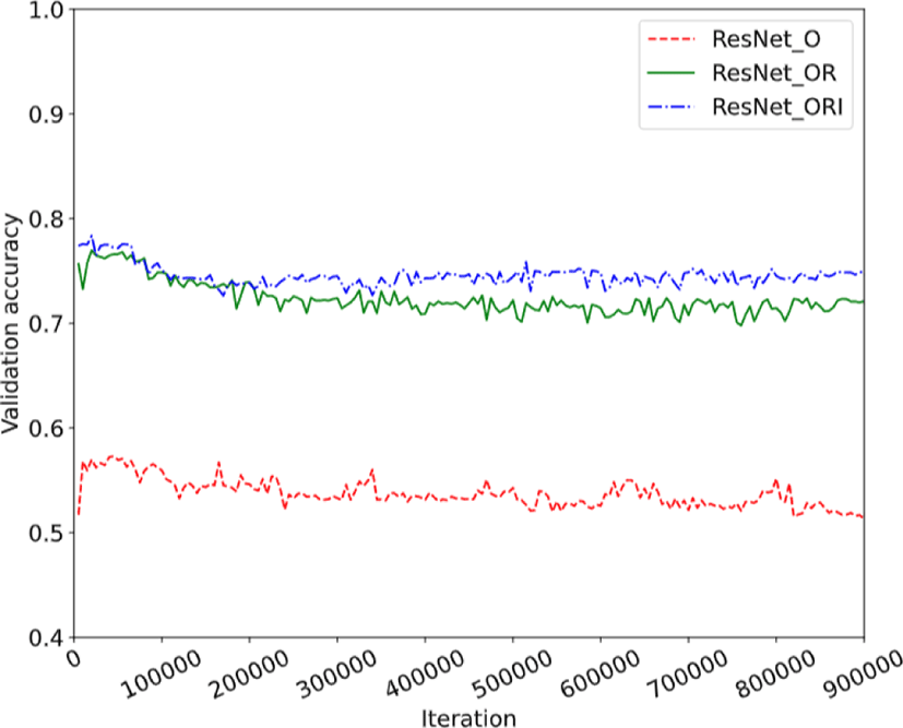
For training the ResNet, the categorical cross-entropy loss was used as the loss function. The weighted categorical cross-entropy loss which was mentioned in Section 3.2 was used for training the MLT-CNN. Figure 15 shows that the proposed MLT-CNN outperforms the ResNet model in terms of validation accuracy. As the MLT-CNN can learn from multiple levels, it can be trained the complex structure of split mode tree.
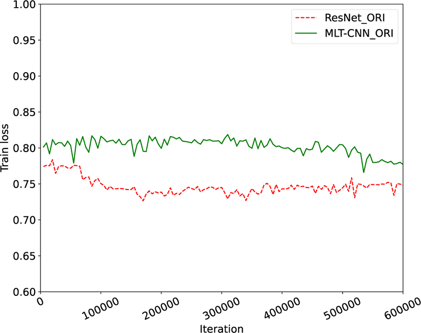
For training the ResNet, the categorical cross-entropy loss was used as the loss function. The weighted categorical cross-entropy loss which was mentioned in Section 3.2 was used for training the MLT-CNN.
Figure 15 shows that the proposed MLT-CNN outperforms the ResNet model in terms of validation accuracy. As the MLT-CNN can learn from multiple levels, it can be trained the complex structure of split mode tree.
In our experiments, all complexity reduction approaches were implemented in the VVC reference software VTM 11.0 [28]. The experiments were conducted on JVET common test sequences [29]. The sequences were encoded as many frames per second (fps) at the random access configuration (using the file encoder_randomaccess_vtm.cfg) at five QP values {22, 27, 32, 37, 42}. After encoding, △T, which denotes the time-saving rate of encoding compared to the original VTM, was recorded to measure the complexity reduction. In addition, the Bjøntegaard delta bit rate (BDBR) was used to assess the RD performance. All experiments were conducted on a system with the same condition in Table 2.
Table 3 shows the BDBR increment and time reduction rate per sequence compared between the proposed method and VTM 11.0 anchor under RA test configuration. For all the sequences, the proposed method achieves 11.53% encoding time saving with 1.01% BDBR increase. The results indicate that the time reduction by the proposed framework happens usually on the high-resolution sequences. This is because there are more CTUs in high resolution sequences. In other words, there are more opportunities for time reduction.
By comparing the 3-rd column and the 4-th column in Table 3, less time reduction occurs on QP 22. Since CUs tend to be split on smaller QPs, it spends more time splitting compared to when encoded with higher QPs, meaning non-split predicted CUs cause more time reduction.
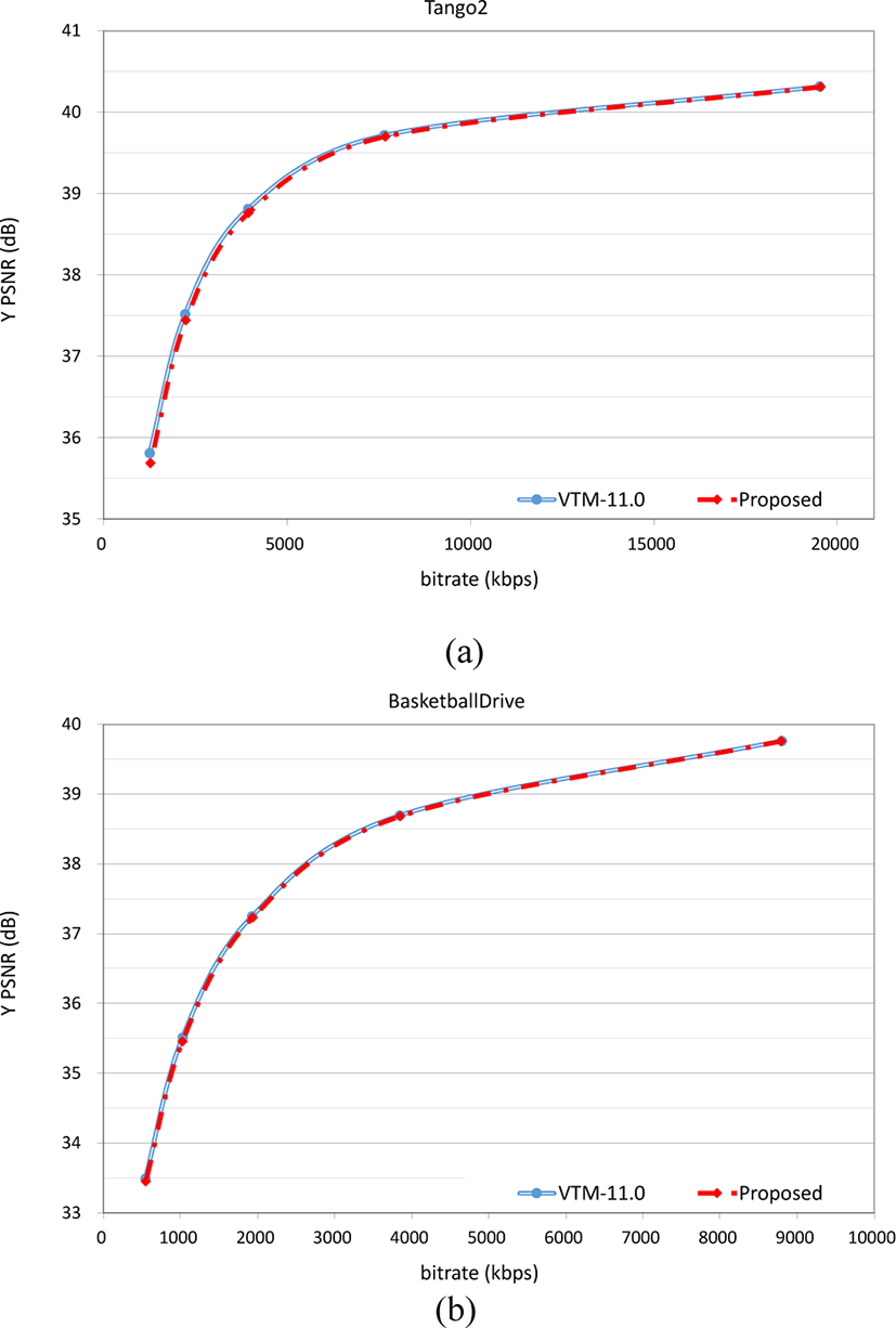
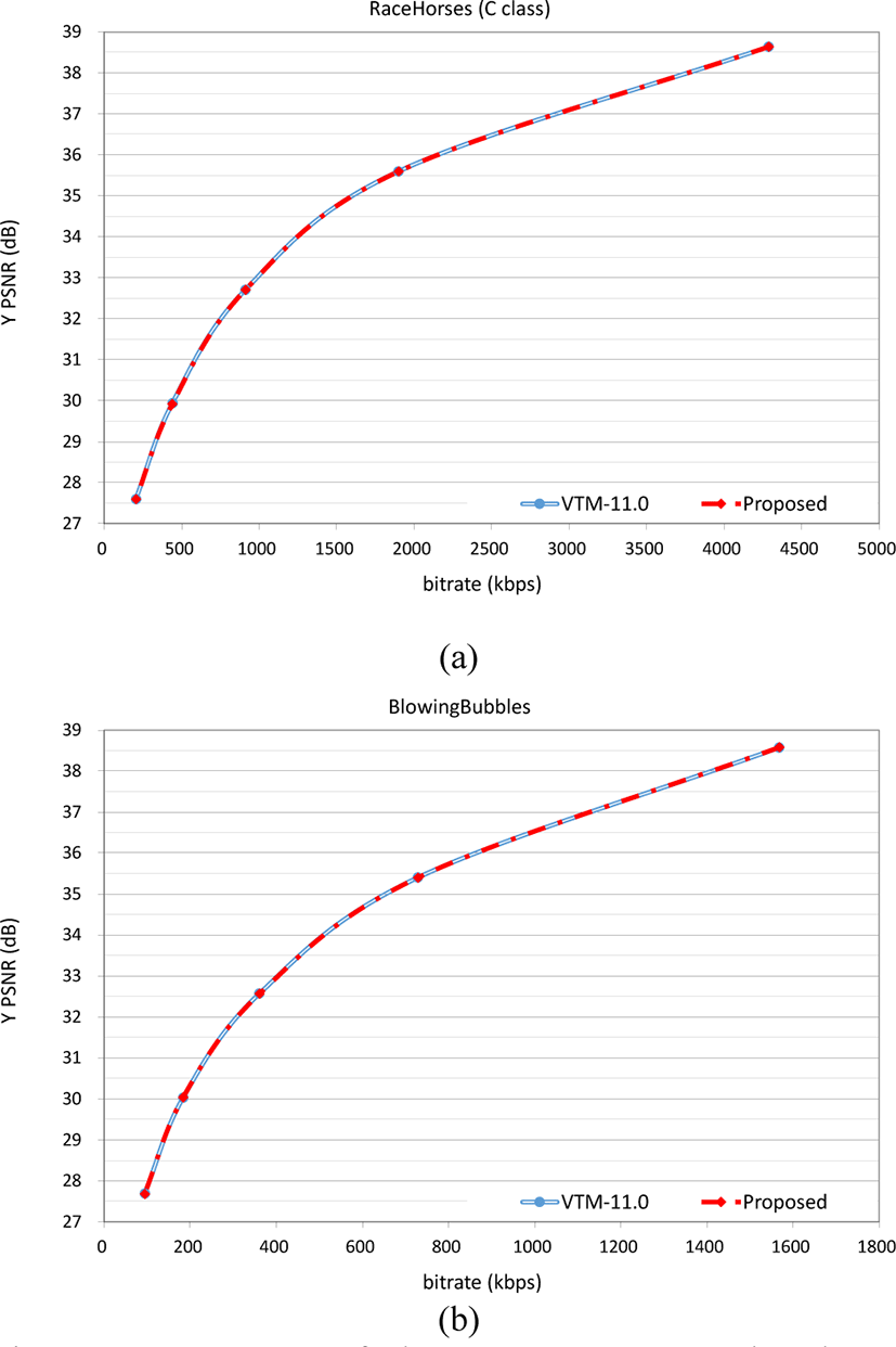
Figure 16 and Figure 17 represent the RD curves of Tango2, BasketballDrive, RaceHorses, and BlowingBubbles sequences. It shows VTM-11.0 and the proposed method have similar RD curves while the proposed method takes less time for encoding. As the MLT-CNN was trained with 128×128 CUs, the same size CUs are aimed in the encoding process.
V. CONCLUSION
In this paper, we have aimed to reduce the time complexity of inter-picture prediction mode as the inter prediction accounts for a large portion of the total encoding time. The problem was defined as classifying the split mode of each CU using the proposed multi-level tree (MLT) CNN. The MLT-CNN reflects the tree structure of six split modes: non-split, quad-tree split, binary-tree horizontal split, binary-tree vertical split, ternary-tree horizontal split, and ternary-tree vertical split. By predicting and computing the loss at each level as in the split mode tree, the network learned complex structure effectively. To improve training performance, we observed the split tendency of CU in different conditions to figure out which information affects split mode. As a result, the original and residual image of a CU, the picture order count (POC), and the CU-level quantization parameter (QP) value were considered. For training MLT-CNN, a dataset that contains the original and residual image, POC, CU-level QP, and the ground-truth of one CU was constructed. In this study, we have targeted 128×128 CTUs. 92 video sequences from the BVI-DVC database were used to build the training and validation set.
The overall algorithm including the MLT-CNN inference process was implemented on VVC Test Model (VTM) 11.0. The sequences were encoded at the random access (RA) configuration with five QPs {22, 27, 32, 37, 42}. The time-saving rate of encoding compared over the original VTM was recorded to measure the complexity reduction. Also, the Bjøntegaard delta bit rate (BDBR) was measured to assess the rate-distortion performance. The experimental results showed that the proposed algorithm can reduce the computational complexity by 11.53% on average, and 26.14% for the maximum with an average 1.01% increase in BDBR. Especially, the proposed method showed higher performance on the sequences of the A and B class, reducing 9.81%~26.14% encoding time with 0.95%~3.28% BDBR increase.
The future work is to improve the performance of robustness on the sequences with different resolutions. MLT-CNN models on 64×64, 32×32, and 16×16 CUs should be combined on the proposed algorithm. Also, the performance analysis on the low delay (LD) configuration is needed to validate the overall performance.




 received her BS degree in the Department of IT Engineering from Sookmyung Womens University, Korea, in 2019. In 2019, she joined the Department of Computer Engineering for pursuing her MS degree at Sookmyung Women’s University.
 (Senior Member, IEEE) received the B.S. degree from Pusan National University, South Korea, in 1996, the M.S. degree from the Korea Advanced Institute of Science and Technology (KAIST), in 1998, and the Ph. D. degree from the Department of Electrical Engineering and Computer Science, KAIST, in 2004. In March 2004, he joined the Real-Time Multimedia Research Team, Electronics and Telecommunications Research Institute (ETRI), South Korea, where he was a Senior Researcher. In ETRI, he developed so many real-time video signal processing algorithms and patents and received the Best Paper Award, in 2007. From February 2009 to February 2016, he was an Associate Professor with the Division of Computer Science and Engineering, Sun Moon University, South Korea. In March 2016, he joined the Department of Information Technology (IT) Engineering, Sookmyung Women’s University, South Korea, where he is currently a Full Professor. He has published over 250 international journal articles and conference papers, patents in his field. His research interests include image and video signal processing for the content-based image coding, video coding techniques, 3D video signal processing, deep/reinforcement learning algorithm, embedded multimedia systems, and intelligent information system for image signal processing.