Autocorrelation Coefficient for Detecting the Frequency of Bio-Telemetry

Nakajima, Isao; Muraki, Yoshiya; Yagi, Yukako; Kurokawa, Kiyoshi

doi:10.33851/JMIS.2022.9.3.233

J Multimed Inf Syst 9(3):233-244

eISSN: 2383-7632

DOI: https://doi.org/10.33851/JMIS.2022.9.3.233

Section D

Autocorrelation Coefficient for Detecting the Frequency of Bio-Telemetry

Isao Nakajima¹^,^*, Yoshiya Muraki¹, Yukako Yagi², Kiyoshi Kurokawa³

Author Information & Copyright ▼

¹Seisa University, Yokohama, Japan, jh1rnz@aol.com, yoshi.muraki@gmail.com

²Memorial Sloan Kettering Cancer Center, New York, NY, USA, yagiy@mskcc.org

³National Graduate Institute for Policy Studies, Health and Global Policy Institute, Tokyo, Japan, kurokawak01@gmail.com

^*Corresponding Author: Isao Nakajima, +81-90-8850-8380, jh1rnz@aol.com

© Copyright 2022 Korea Multimedia Society. This is an Open-Access article distributed under the terms of the Creative Commons Attribution Non-Commercial License (http://creativecommons.org/licenses/by-nc/4.0/) which permits unrestricted non-commercial use, distribution, and reproduction in any medium, provided the original work is properly cited.

Received: Sep 11, 2022; Revised: Sep 25, 2022; Accepted: Sep 26, 2022

Published Online: Sep 30, 2022

Abstract

A MATLAB program was developed to calculate the half-wavelength of a sine-curve baseband signal with white noise by using an autocorrelation function, a SG filter, and zero-crossing detection. The frequency of the input signal can be estimated from 1) the first zero-crossing (corresponding to ¼λ) and 2) the R value (the Y axis of the correlogram) at the center of the segment. Thereby, the frequency information of the preceding segment can be obtained. If the segment size were optimized, and a portion with a large zero-crossing dynamic range were obtained, the frequency discrimination ability would improve. Furthermore, if the values of the correlogram for each frequency prepared on the CPU side were prepared in a table, the volume of calculations can be reduced by 98%. As background, period detection by autocorrelation coefficients requires an integer multiple of 1/2λ (when using a sine wave as the object of the autocorrelation function), otherwise the correlogram drawn by R value will not exhibit orthogonality. Therefore, it has not been used in bio-telemetry where the frequencies move around.

Keywords: Frequency-Voltage Conversion; Orthogonality; Zero-Cross; Savitzky-Golay; Hawkmoth Receiver

I. INTRODUCTION

Frequency-to-voltage (F/V) conversion, the ability to obtain an output voltage proportional to a frequency input, is an important basic electronic technology whose applications include speed control, flow measurement, tachometers, Doppler radar for speed sensing, and touch or sound switches [1].

Medical telemetry, which collects electrocardiograms and respiratory patterns from patients lying on a bed with a small device and transmits them remotely, such as to nursing stations, is also an indispensable device in hospitals around the world [2-10]. Before the era of packet transmission through AD converter, many of these devices convert the electrocardiogram of a patient from voltage to frequency, and transmit it by frequency-modulated (FM) waves to obtain a sufficient signal-to-noise (S/N) ratio. Specifically, the electrocardiogram signal is modulated as a voice-band FM signal, and the voice-band signal is transmitted by 450-MHz-band FM waves. This is because the S/N ratio required by the F/V conversion element on the receiving side is high.

Unlike the 12-lead electrocardiogram, the amount of information required by the patient monitoring device is not required to depict subtle ST-segment changes, so the amount of information is such that events are included with an analog-to-digital (A/D) converter that acquires 250 samples per second. Considering Nyquist’s theorem, information that can be stored in a 500-Hz band is transmitted in an occupied band of 8 kHz to 450 MHz, meaning that some of the frequency resource is wasted.

In our hawkmoth transmitter, we convert the analog potential of the electromyogram (EMG) into frequency, so the receiving side is required to have a function to obtain a potential proportional to the frequency change. Therefore, this paper describes two methods that do not use FM double modulation. Specifically, the transmitting side performs one V/F conversion, and the receiving side receives the signal as a single side-band (SSB) signal with white noise instead of receiving it in FM. We are considering a method of using digital signal processing (DSP) technology to obtain the frequency from the received signal, and assign a suitable voltage from a lookup table for frequency/potential conversion. Frequency detection and vacant channel detection using the autocorrelation function are also being studied in the field of communications [11-12]. Based on these reports, here we convert the received telemetry signal into a baseband denoised signal with an autocorrelator.

The V/F function of digital processing, which is remarkably effective in denoising and can discriminate even if the frequency is variable, can be used in the future to receive analog signals from micro devices that do not have CPUs nor packet transmitters. For example, if a transmitter with a V/F function with the size of a grain of rice can be inserted directly into the myocardium via a thoracic endoscope and the heartbeat vibration can generate electricity, it will continue to transmit weak noise-level radio waves. If it were attached at the myocardium near the pulmonary venous and send voltage data of the cell, it can be used to predict the atrial fibrillation and to develop drugs that prevent its onset. Applications for in vivo microtechnology are limitless.

In view of such a future, we report the comparison verification of an analog F/V conversion device and digital conversion simulated by MATLAB. We also discuss the reduction of the computation and future prospects related to autocorrelation with polyphase methods.

II. PRINCEPLE

Here, we adopted a method of demodulating the signal using the autocorrelation function, detecting the frequency from the zero-crossing, and giving the corresponding voltage as a digital conversion of the F/V. In this section, we mathematically explain the basis, the norm, the Fourier spectrum by fast Fourier transform (FFT), the power spectrum density function (commonly known as the power spectrum), and the angular velocity ω stored in the autocorrelation of the sine wave.

2.1. Definition of Norm

For each vector in the complex vector space, we define the norm by the inner product (|| ||) (equation (1)). At this time, three properties (equations (2)–equations (4)) hold.

‖ V ‖ = (V, V) 1 / 2 .

(1)

‖ V ‖ ≥ 0, ‖ V ‖ = 0 ⇔ V = 0.

(2)

‖ a V ‖ = | a | ‖ V ‖ .

(3)

‖ V + y ‖ ≤ ‖ V ‖ + ‖ W ‖ .

(4)

Mathematical definition of period can be defined as follows. If f(t) is assumed to be the magnitude at time t, for a continuous and periodic signal, at a later time nT, f(t)=f(t + nT).

In reality, the received signal is not completely equal, but generally has such a property, and this function is called a periodic function of period T. For the sine function, the period is T=1/(2πf). In this paper, for the purpose of discriminating the frequency of the sine curve using DSP (e.g., FFT and inverse FFT, or IFFT), this period T is such that f(t) = f(t + nT).

The purpose is to obtain the frequency of the sine curve using the autocorrelation function.

In general statistics, in a correlogram, which is a trendgram of the autocorrelation coefficient R, one datum shifted by time Δt is called a lag. Therefore, it is called a sample instead of a lag, and the address AAA is used to express the X-axis address of the correlogram. A single sine curve containing white noise and a signal are output from an A/D conversion device with a sampling rate of XX (Hertz or Sampling Per Second). This signal is taken in a certain window and mathematically processed. In this paper, this window is called a “segment” to distinguish it from the frame size used in FFT. The FFT frame size is 2ⁿ times larger, but the segment can be freely resized to improve frequency discrimination.

The spacing of the samples before processing is kept constant, but the time between samples in the segment after autocorrelation processing is not evenly spaced, and the orthogonality of the Y- and X-axes of the correlogram is not preserved. In other words, the multiple samples are arranged in chronological order within the segment, but the relationship between the Y-axis and the X-axis of the correlogram is distorted. Under certain conditions (e.g., when the segment size is an integer multiple of half the wavelength of the frequency of the input signal), the intervals between samples are equal. Conversely, it is possible to focus on this sample sequence with large temporal distortion and use it for frequency discrimination.

The segments are of variable length. Specifically, if the A/D conversion sampling rate is 1 MHz, 1,000,000 samples are output per second. If one segment consists of 4,000 samples, we can divide the data into 250 segments per second, so we can detect 250 frequencies per second.

2.2. Definition of Autocorrelation Function

The autocorrelation function Rff after time τ in the function f is defined as in equation (5). At this time, the inner product of the function (equation (6)) and the norm can be written as equations (7) and equations (8).

Rff (τ) = (f (t), f (t + τ)) / ‖ f (t) f (t + τ) ‖ .

(5)

((f (t), f (t + τ)) = ∫ t 0 t 1 f (t) f (t + τ) d t .

(6)

‖ f (t) ‖ = ∫ t 0 t 1 f (t) 2 d t .

(7)

‖ f (t + τ) ‖ = ∫ t 0 t 1 f (t + τ) 2 d t .

(8)

The correlation coefficient R (from -1 to +1) between the functions f(t) and f(t+τ) is calculated. In the specific arithmetic processing, whether to divide by the lag or subtract the mean value of the function depends on the result after the experimental arithmetic processing. In other words, is periodicity required from the results? “What is the cycle?” Is it possible to further remove aperiodic noise? “What is the S/N ratio?” These are the evaluations of the calculation process. Basically, periodicity has a high degree of approximation, and noise removal (non-periodicity) has a greater effect.

When used for predicting sunspots, for example, it is better to obtain the lag of each point of the linear function of f(t), but this is not suitable for high-speed processing of the sine function. We recommend the following power spectrum method using FFT and IFFT.

2.3 Autocorrelation Function by Power Spectrum

Because the received signal is based on a sine function and its continuity and periodicity are self-evident, we attempted to apply an autocorrelation function using the power spectrum, and developed mathematical logic accordingly. In this section, the received signal is described as g(t) to distinguish it from the above method.

The Fourier transform is defined (equation (9)) as the Fourier integral g(f). Furthermore, its inverse transform g(x) is represented by equation (10). The signal g(x) is often a real number, but g(f) is generally a complex number, and the square of its absolute value is called a power spectrum. This power spectrum is expressed as in equation (11), where * represents a complex conjugate. This IFFT is equation (12), which is obtained from equation (8) and equation (10).

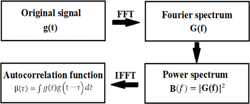
The power spectrum of the signal g(t) is obtained as the square of the absolute value of the FFT. Furthermore, because the IFFT is the norm of equations (10) and (12) with respect to the function at time τ, equation (13) is obtained by applying IFFT to the power spectrum of the FFT. This will yield the self-correlation R on the time axis. The concept of the relationship between power spectrum and autocorrelation function is shown in Fig. 1.

Fig. 1. Relationship between power spectrum and autocorrelation function. Note: The power spectrum density function is generally called the power spectrum. This is because it is linear with the waveform that can be observed with a commercially available frequency spectrum instrument, and the value obtained by multiplying the power spectrum density function by the bandwidth (Hz) is the same. In this paper, since we are comparing t=0 and t=τ, the frequency components cancel out. The power spectrum density function is treated same as the power spectrum. If the power spectrum density function is IFFT-processed, the autocorrelation function is calculated. Conversely, if the autocorrelation function is FFT-processed, the power spectrum density function is obtained. The two form a pair in the Fourier transform, and this relationship is called the Wiener-Khinchin theorem.

Download Original Figure

G (f) = ∫ − ∞ + ∞ g (t) exp (− 2 π i t f) d t .

(9)

g (t) = ∫ − ∞ + ∞ G (t) exp (2 π i t f) d f .

(10)

B (f) = | G (f) | 2 = G (f) G (f) * . * Complex conjugate .

(11)

β (τ) = ∫ − ∞ + ∞ B (f) exp (2 π i f t) d f .

(12)

β (τ) = ∫ − ∞ + ∞ g (t) g (t − τ) d t .

(13)

As an advantage, FFT peak detection may erroneously detect double or triple frequencies, but the peak of the autocorrelation function can stably determine the fundamental frequency. The reason is that the frame size of the Fourier transform does not appear in the formula for calculating the peak of the autocorrelation function.

2.4. Preservation of Angular Velocity in the Sinusoidal Autocorrelation Function

Because the autocorrelation Rff (τ) of the sine wave is the product of the sine wave separated by time τ, it is expressed as equation (14), which is transformed to obtain equations (15), (16), and (17). Because the ratio of integration against τ=0 is the correlation coefficient R, finally equation (19) is obtained. equation (19) means that the autocorrelation function of a sine wave is expressed as the cosine of an even function, and more importantly, the equivalency of its angular velocity ω to the frequency is preserved. In this paper, we use this characteristic to estimate the frequency (only single sinusoidal waves) received by telemetry from the autocorrelation coefficient R.

Rxx (τ) = lim T → ∞ 1 T ∫ − T 2 T 2 s i n ω t s i n ω (t − τ ） d t .

(14)

= lim T → ∞ 1 T ∫ − T 2 T 2 sinωt {sinωt cosωτ − cosωt sinωτ} d t .

(15)

= lim T → ∞ 1 T ∫ − T 2 T 2 sin 2 ωt cosωτ − sinωtcosωt sinωτ} dt .

(16)

= lim T → ∞ 1 T ∫ − T 2 T 2 1 − c o s 2 ω t 2 c o s ω τ − s i n 2 ω t 2 s i n ω τ} d t .

(17)

= lim T → ∞ 1 T ∫ − T 2 T 2 {c o s ω τ [t 2 − s i n 2 ω t 4 ω] T / 2 ＋ s i n ω τ [− c o s 2 ω t 4 ω] T / 2} .

(18)

lim T → ∞ 1 T (T 2 c o s ω τ) = c o s ω τ 2 .

(19)

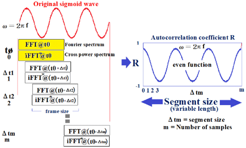
As shown in equation (13), the autocorrelation is the product of the IFFT function of the power spectrum and the product of time zero and the function separated by time τ. This is repeated m times from time zero (maximum value of τmax), and trial waveforms are drawn. The size of the frame containing the sample is called the segment size (or segment length). If the segments are integer multiples of half-wavelengths of the original frequency, the angular velocity ω is preserved in the correlogram. To obtain the power spectrum, the current signal is sampled at multiples of 2², and this size is called the frame size. Fig. 2 shows the relationship between the original signal and the autocorrelation function, and the concept of the FFT frame size and autocorrelation segment size. The segment size can be chosen to optimize the frequency discrimination according to the frequency of interest.

Fig. 2. Relationships between the original signal and autocorrelation function, and between the segment size and frame size of the FFT. Note: That segments 0, 1, 2, and 3 do not change order, but they are not evenly spaced. The only time the autocorrelation coefficient R diagram, X-axis, and Y-axis are orthogonal is when the segment size is an integer multiple of the half-wavelength of the original signal. Otherwise, the X- and Y-axes are distorted.

Download Original Figure

III. METHODS

3.1. Simulation

The biological telemetry assumed here converts a biological signal (potential of, e.g., an electrocardiogram or EMG) into potential and frequency (modulation) and transmits it as radio waves. Then, the receiving side receives the signal secured by the receiving antenna as a SSB. It is demodulated as a baseband (voice band) by the machine.

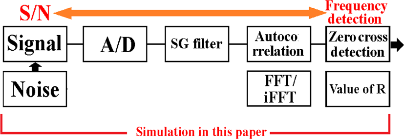
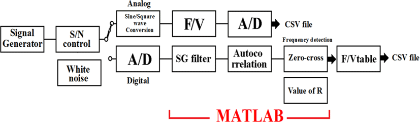
The demodulated signal is a sine wave with white noise and the objective is to find its frequency. This is because the potential of the biological signal can be obtained from the frequency. The function of the block diagram shown in Fig. 3 is described in MATLAB (February 2018 version) as a simulation of frequency detection using the autocorrelation function. Because the S/N ratio is used as a parameter, variable white noise is added, and the sine curve signal is passed through a Savitzky-Golay (SG) filter [13-14], after some degree of denoising, and then the autocorrelation coefficient R is calculated as a cosine function within the segment using correlograms. For frequency discrimination, the zero-crossings on the correlogram are detected, the amplitude of R (value of R) at the center of the segment is obtained, and the correlation between the first zero-crossing address and ¼λ of the actual frequency within the segment is obtained. A block diagram of the functions used in the simulation is shown in Fig. 3, and a summary of the MATLAB functions used is shown in Table 1.

Fig. 3. Block diagram showing simulation functions.

Download Original Figure

Table 1. Major MATLAB functions used in the simulation.

Functions	Content
awgn(m,n,power)	Create white noise
sgolayfilt(x,order,framelen)	Savizky-Golay filter using cubic (3 order) 49 points
fft(X,n)	Fourier transform
ifourier(F,transVar)	Inverse Fourier transform
power=Y.*conj(Y)	Power spectrum
auto_y=real(ifft(power)); auto_y = auto_y./max(auto_y);	Autocorrelation is defined as the product of the shifted amount
zeroCross=auto_y(1:end-1).*auto_y(2:end) < 0;	Get the zero cross point
SNR = snr(y);	Calculate the signal S/N

Download Excel Table

3.1.1. Original Signal Condition

In this article, the purpose is to reproduce FM telemetry signals, and the original signal received by the SSB receiver must meet the following conditions for this simulation to hold:

Only one sine wave with white noise is processed.
There are no other periodic interfering waves, and of course any noise has no periodicity.
The frequency change of the signal is continuous, and the frequency difference from the previous segment is small (frequency fluctuation is less than a few percent).
The amplitude of the signal is nearly constant within the segment.

3.1.2. Savitzky-Golay Filter

For noise removal, a SG filter is used to prevent deviation of the time axis from the peak values. Finite impulse response is also acceptable, but when measuring multiple channels at the same time, for example, when measuring EMG1 and EMG2, if the finite impulse response coefficients are different, the peak timing will have an error. The noise elimination function is also important, but we want to minimize time axis deviations and phase differences in this system because a phase difference can lead to a potential difference in F/V conversion.

3.1.3. Basic Concept

The basic program operation is to take m samples in a segment and apply the autocorrelation function. Because the signal contains white noise (left side of Fig. 4), the power spectrum at this time is the center of the correlogram. The maximum value of R is the first or last ¼λ cosine wave extremum (estimated by an approximation formula).

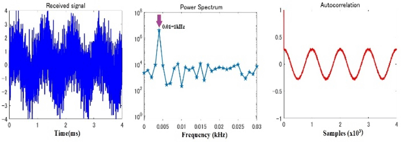
Fig. 4. Noise and signal (left), frequency spectrum obtained by FFT (center), and correlogram obtained by the autocorrelation function (right). The sampling frequency is 1 MHz, with 4,000 samples/segment.

Download Original Figure

The X-axis of the power spectrum is frequency, and when the noise level is low and a peak value can be obtained, it roughly indicates the frequency of the original signal. However, because the X-axis is logarithmic (multiple of 2²), the frequency discrimination ability is poor at low frequencies (center of Fig. 4). However, when an autocorrelator is used, the segment size can be selected according to the target frequency, which allows us to select the length that increases the frequency discrimination ability. In addition, because autocorrelation provides a high denoising effect (right side of Fig. 4), the frequency resolution is dramatically improved compared to that of power spectrum peak detection.

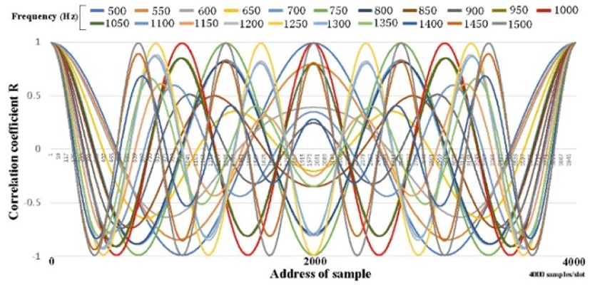
3.1.4. Frequency Discrimination by Amplitude at Center Address

One wave of a signal input at 500–1,500 Hz (intervals of 50 Hz) can be drawn as shown in Fig. 5 by taking the autocorrelation with 4,000 samples/segment at a sampling rate of 1 MHz. For all input vibrations, the maximum value of R is the first or last ¼λ cosine wave extremum (estimated by an approximation). Even if the S/N ratio deteriorates, the waveform is similar and becomes smaller, but the maximum value of R is the maximum immediately after the correlation is started or immediately before it ends. All waveforms are even functions and are symmetrical at the center address, which is 2,000.

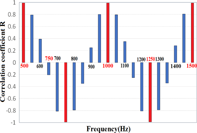
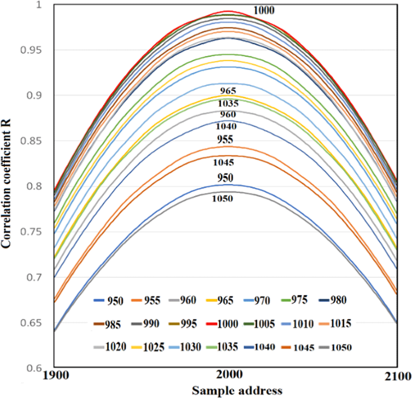
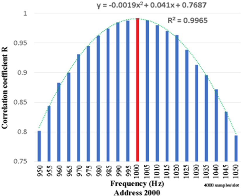
Fig. 5. Waveforms drawn from autocorrelation of a single wave of a force signal input at 500–1,500 Hz (intervals of 50 Hz) in one segment with 4,000 samples with an A/D conversion rate of 1 MHz.

Download Original Figure

Because it is an even function, we should pay attention to the value of the center address, 2000. At each frequency, as shown in Fig. 6, the magnitude of R is different, but the S/N ratio deteriorates, and the R wave has a small amplitude overall. Even if it becomes a wave, the maximum value R can be grasped by the method described above, and it can be normalized as 1 (Fig. 6). Furthermore, the value of R at the center address of 1,900–2,100 Hz can be drawn in detail as shown in Fig. 7, and of 950–,1050 Hz as shown in Fig. 8. The amplitude of R at the center address is determined by the relationship between the frequency and the segment. If the segment size is an integer multiple of the input half-wavelength, R is 1 even at the center address, and the other frequencies are as shown in Figs. 6, Figs. 7, and Figs. 8. Because the amplitude of the value of the center address R depends on the frequency, this point is an effective factor to increase the frequency discrimination.

Fig. 6. Relationship between R values and frequency 500–1,500 Hz at the center (Sample address 2000). At frequencies where periodicity is maintained, R=1 (logical value) is ensured, which is the definition of autocorrelation.

Download Original Figure

Fig. 7. Center of the segment at 1,900–2,100 Hz for estimating the frequency from the R value at 950–1,050 Hz.

Download Original Figure

Fig. 8. Center of the segment at 950–1,050 Hz for estimating the frequency from the R value.

Download Original Figure

The frequency can be estimated by the approximation formula of the quadratic function.

3.1.5. Frequency Discrimination by Zero-Crossing Address (¼λ)

Fig. 9 shows the correlation between the first zero-crossing of the correlogram and each frequency. If the segment size is an integer multiple of the input half-wavelength, the zero-crossing obtained in the simulation will coincide with the logical value of ¼λ of the input frequency. Similarly, the amplitude of each wave takes the maximum value of R, and the orthogonal relationship between the Y-axis and the X-axis is established, but the coordinates are distorted at other frequencies.

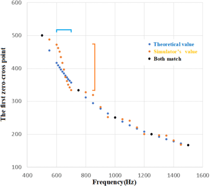
Fig. 9. Parts with large distortion are suitable for frequency discrimination. In this case, 600–700 Hz is a suitable target frequency (4,000 samples/segment).

Download Original Figure

As the input frequency increases, more waves are included in the segment, and the difference between the first zero-crossing obtained in the simulation and the logical value gradually decreases. However, one frequency can be obtained from one segment, so a long segment size decreases the temporal resolution of the biological signal. What is important here is to use a portion with a large dynamic range for frequency discrimination even if the coordinates are distorted. Specifically, the zero-crossing value changes greatly, but, conversely, if the difference between the input frequencies is small, the frequency discrimination ability increases.

As shown in Fig. 9, the first zero-crossing changes greatly for input frequencies of 600–700 Hz, so this portion is used for frequency discrimination. Fortunately, the segment size can be serially passed backwards as information, so the previous frequency is available for backward processing. By varying the segment size based on this information, for example, the segment size can be adjusted to target frequencies corresponding to a segment size of 4,000, or 600–700 Hz (median 650 Hz). In other words, if the previous frequency is 1,300 Hz, the segment size is 2,000, and if the previous value is 1,500 Hz, the segment size is 1733. This can improve the frequency resolution. However, because the part corresponding to 600–700 Hz is not an integer multiple of a half-wavelength, in the above procedure, R will not be 1, but the part corresponding to 600–700 Hz will be affected if the S/N ratio deteriorates. The frequency discrimination is higher than the value of R at the center address.

3.1.6. Reduce Computation by 98%

The sample corresponding to the lag of the correlogram is the value of the multiple integral obtained by performing FFT and IFFT, and the X axis has similar values to the right and left via center line, but mathematically they are independent.

In general, even if there are no adjacent values, the R value can be obtained by calculating against FFT*iFFT of the coordinate zero as one coordinate on the correlogram. However, MATLAB functions do not process if the intervals between the matrix are not uniform, so here we will explain under the condition that the intervals between the segments of 0–2,000 are uniform.

We are interested in the zero crossing of 1/4λ, the amplitude of the central cosine wave (R value), and the amplitude of the cosine wave near the end (R value). It is assumed here that the 2,000-sample waveform of the segment already has a table of correlograms at various S/N levels on the CPU side as a reference. In other words, reducing the number of calculations means, "How far can we reduce the number of samples from 2,000 samples?" Is it possible to maintain the frequency discrimination ability and withstand actual use? is. If the computational processing is lowered, the discrimination ability will be lowered, so it is a conflict with the needs.

In order to visually understand this theme, Fig. 10 shows the correlogram when it is temporarily reduced from 2,000 samples to 40 samples (41 calculations because there are actually zeros shown in green allow).

Fig. 10. Reduce computation by 98%.

Download Original Figure

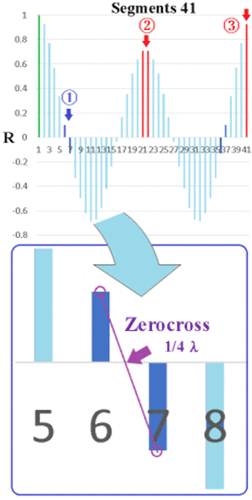
The points to watch are arrows 1, 2, and 3. The first 1 is the 1/4λ zero crossing, and the coordinates of the zero crossing are obtained using the auxiliary line. Arrow 2 is the median value of the sample, and there are two values, but since it is an even function, they are almost the same value. The third arrow obtains the R value near the end in order to obtain the reference value of the R value with S/N. From this 1, 1/4λ is obtained, and from 2 and 3, two candidate λs are obtained (one value is close to 1/4λ, the rest are imaginary). As a result, the number of calculations for FFT and IFFT is reduced to 2001 or 41, and the calculation reduction rate is 98% reduction, and the remaining 2% should be calculated. Furthermore, if it is 41 segments, Savitzky-Golay (third order, 17 points) can be used, and there is also a denoising effect.

In this way, the autocorrelation coefficient R for a sine curve can always be drawn as a cosine and becomes an even function that folds back at the median. With this in mind, as mentioned above, it is also possible to cut 41, 98% reduction of the FFT calculation from 2001, lighten the CPU and DSP calculations, and pave the way for implementation.

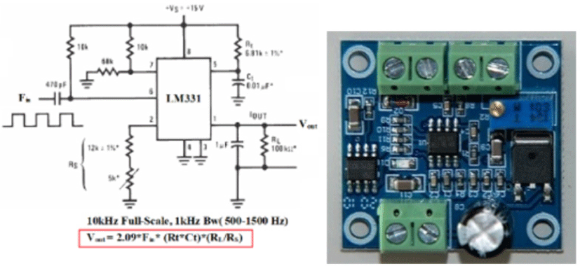
3.2. Comparison of Analog and Digital Processing

3.2.1. Comparative Experiment

We generated a stable 1,000-Hz signal from a signal generator, added white noise, changed the S/N ratio, added noise to the analog element, recorded the resulting voltage with a sampling speed of 500 kHz, processed the potential with a 16-bit A/D conversion, and recorded the result in a CSV file. On the digital side, A/D conversion was performed under the same conditions, the data were imported into MATLAB on a PC, and the frequency component of the autocorrelation coefficient R was obtained and recorded in a file. Then, these two files were compared. A block diagram of the evaluation experiment is shown in Fig. 11, and Fig. 12 shows the F/V converter circuit diagram and board used in the analog circuit.

Fig. 11. Block diagram of evaluation with analog elements and digital processing by autocorrelator and Savitzky-Golay filter.

Download Original Figure

Fig. 12. Analog circuit F/V conversion device LM331: Circuit diagram (left) and device mounted on a circuit board (right).

Download Original Figure

3.2.2. Measurement Result

A comparison of the two measurements is shown in Table 2. The F/V conversion element calculated the frequency from the potential fluctuation. The length of the 1,000-Hz signal was 400 ms, 400 segments were measured, and the standard deviation was obtained. The S/N ratio of 8 dB in the F/V conversion circuit is almost equal to the autocorrelation function of –14 dB, with a standard deviation of ±4, and the difference is 22 dB. A standard deviation of ±4 Hz is the limit for practical use.

Table 2. Relationship between the S/N ratio and standard deviation of error (Hz).

Input frequency 1,000 Hz	S/N (dB)	Standard deviation of error (Hz)
F/V analog device	+20	+/−0.2
F/V analog device	+8	+/−4.1
Autocorrelation+SG	+8	+/−0
	−11	+/−1.8
	−14	+/−4.0

Download Excel Table

3.2.3. Comparison with Actual Data

Using a chicken electrocardiogram, we compared the signal before V/F conversion, the demodulation by the analog F/V element, and output from the digital processing autocorrelator (250 segments/second) (Fig. 13). As for the V/F frequency characteristics on the transmitting side, the dynamic range peaks at high frequencies, so the R-wave head is suppressed. Even so, the autocorrelation function does not clearly show high amplitude in the R wave, but this is because a SG filter is applied to improve the S/N ratio. Unlike FIR, the SG filter does not generate a temporal delay in the amplitude, but the amplitude drops to some extent. Similarly, the amplitude of the R wave is also falling in the F/V element, but this is because it is a low pass filter due to the effect of the time constant added in parallel to the output.

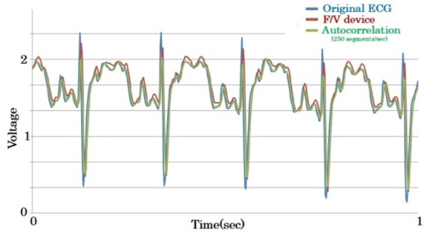
Fig. 13. comparison with analog F/V device and autocorrelator (250 segments).

Download Original Figure

Even if the above exclusions are taken into account, it is clear that the R wave is still significantly pumped in autocorrelation and cannot follow a frequency that rises instantaneously. This shows the limitation of analyzing only one segment, and to solve this, we should incorporate forward prediction by deep learning based on past data, and implement a parallel computing method by polyphase and multiple-segment operation.

IV. CONSIDERATIONS

4.1. Improved Frequency Discrimination

In this study, the band of the transmission frequency was relatively narrow at 1 kHz, so the SSB baseband frequency was 500–1,500 Hz. Theoretically, only 500 pieces of information per second can be carried in a 1-kHz band according to Nyquist’s theorem, so a frequency resolution of 2 Hz is sufficient. In addition, the fluctuation of the autocorrelation function, based on its standard deviation, is ±2 Hz, so the resolution is 4 Hz, or 250 segments/second. [Please verify that the editing is consistent with your intended meaning.] To increase the resolution of the potential axis in the future, it is necessary to improve the following conditions:

Increase the frequency band on the transmitting side. For example, if 0.01V is 4 Hz, and this is changed to 40 Hz, the error of 4 Hz becomes 0.001 V.
Widen the baseband frequency band of the SSB receiver. For example, if the band is increased from 500–1,500 Hz to 2,500–3,500 Hz, the frequency resolution will triple. In this case, a software DSP receiver (software-defined radio receiver) is more suitable than an SSB receiver, whose reception band is fixed by a crystal filter.
Increase the number of A/D converters working in parallel. By increasing the number of A/D conversion elements and attaching an autocorrelation function to process them, the frequency resolution will increase.

Rather than converting the input signal from analog to digital and passing this data string to the DSP field-programmable gate array (FPGA) after time-sharing, multiple A/D converters are arranged in parallel and operated with a time difference, and the autocorrelation function is used in each calculator to find the R values at zero-crossings and segment centers to speed up the process. If the segment can be varied by passing information on the frequency of the preceding segment to the subsequent calculation unit, high frequency discrimination ability can be obtained.

4.2. Road to Implementation

4.2.1. Subjects

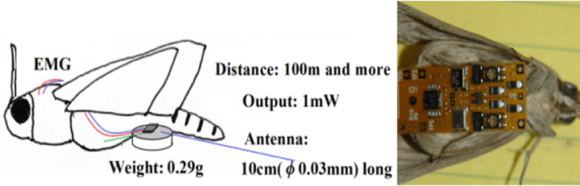
For research subjects that cannot carry a CPU, such as moths, butterflies, and sparrow-sized birds, the payload is limited, the battery is limited, the transmission power is small, and the antenna is small, resulting in an extremely small effective isotropic radiated power (EIRP) [Please verify that I defined EIRP correctly.] (Fig. 14). Therefore, it is not easy for the receiving side to obtain a sufficient S/N ratio. In conventional biotelemetry transmission, both primary and secondary modulations are frequency conversions, occupying a wide frequency band and not effectively using frequency resources. Note that the existing method uses a large transmission power.

Fig. 14. Bio-telemetry of 2-channel EMGs for a moth subject.

Download Original Figure

For small subjects, such as moths, butterflies, and small birds, our proposed digital processing (autocorrelation function) enables efficient use of frequencies and reproduction even when the S/N ratio is low [15-18].

4.2.2. Parallel Processing with Polyphase

Polyphase segment processing is a method of detecting frequencies by running multiple segments at the same time. A handling protocol is required to distribute data from the A/D converter to multiple computing units. In this way, the processing time can be shortened.

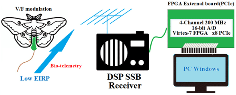
What elements are needed to implement the above algorithm? The specific proposal here is the FPGA + A/D board, Model 78760 (PC expansion board for Windows). This board is a PCI Express board with 200-MHz 16-bit 4-channel ADC and a Virtex-7 FPGA. As mentioned above, the autocorrelation functions are only general-purpose FFTs and IFFTs, so the design is easy, and processing three autocorrelation functions in parallel does not pose a problem in terms of capacity. Because 4-GB DDR3 SDRAM is mounted on this board as an external memory for the FPGA, it is also possible to store data temporarily. The host interface is a PCIe x8 lane, through which data can be transferred to Windows at high speed (Fig. 15). By inserting a board with an FPGA capable of four self-functions and a 4-channel A/D converter into the expansion bus of the PC, the frequency discrimination ability will improve fourfold in the time axis direction.

Fig. 15. Conceptual diagram of the entire system and FPGA board for future implementation.

Download Original Figure

Autocorrelation functions using power spectrum require high-speed calculations, so there have been reports of FFT, iFFT and related processing being implemented in FPGA. The reported implementations are extremely helpful for this research [19-22].

V. CONCLUSION

A MATLAB program was developed to calculate the half-wavelength of a sine-curve baseband signal with noise by using an autocorrelation function, a SG filter, and zero-crossing detection. The frequency of the input signal can be estimated from 1) the first zero-crossing (corresponding to ¼λ) and 2) the R value at the center of the segment. Thereby, the frequency information of the preceding segment can be obtained. If the segment size were optimized, and a portion with a large zero-crossing dynamic range were obtained, the frequency discrimination ability would improve.

Using an FPGA board with multiple A/D converters and multiple high-speed computing units makes it possible to quickly transfer the information of the previous segment backwards, allowing the algorithm to be implemented in Windows.

ACKNOWLEDGMENT

We wish to thank Professor Noriyasu Ando of the Maebashi Institute of Technology, who provided the moths used in the present study. This experimental research was performed with assistance from Ms. Miyoshi Tanaka and Ms. Hiroko Ichimura of Nakajima Labo, Tokai University, and Mr. Kokuryo Mitsuhashi and Ms. Megumi Amano of Seisa University. The flexible board of the transmitter was assembled by Japan System Design Inc., Hiroshima City, Japan. This research has resulted in a patent application by Tasada Works Inc., Takaoka City, Japan.

REFERENCES

[1].

M. P. Prajakta and G. Ramachandran, "Electrocardiogram telemetry," in IEEE the 3rd International Conference on Electronic Computer Technology, Apr. 2011, pp. 8-10.

[2].

H. Nakajima and T. Shiga, "Systems health care," in Proceeding of IEEE SMC, Oct. 2011, pp. 1167-1172.

[3].

W. Roel and M. John, "Comparing spectra of a series of point events particularly for heart rate variability data," IEEE Transaction on Biomedical Engineering, no. 4, pp. 384-387, Apr. 1984.

[4].

S. Yazaki and T. Matsunaga, "Evaluation of activity level of daily life based on heart rate and acceleration," in Proceedgings of SICE Annual Conference 2010, Aug. 2010, pp. 1002-1005.

[5].

K. Itao, T. Umeda, G. Lopez, and M. Kinjo, "Human recorder system development for sensing the autonomic nervous system," in Proceeding of IEEE Sensors, Oct. 2008, pp. 423-426.

[6].

K. Itao and T. Ito, "Integrated sensing systems for health and safety," in 2011 Symposium on Design, Test, Integration & Packaging of MEMS/MOEMS (DTIP), May 2011, pp. 212-216.

[7].

H. Kim, R. F. Yazicioglu, and S. Kim, "A configurable and low-power mixed signal SoC for portable ECG monitoring applications," in VLSI Symposium, Jun. 2011, pp. 142-143.

[8].

S. Y. Hsu, Y. L. Chen, and P. Y. Chang, "A micropower biomedical signal processor for mobile healthcare applications," in Proceeding of IEEE ASSCC, Nov. 2011, pp. 301-304.

[9].

M. Ashouei, J. Hulzink, and M. Konijnenburg, "A voltage-scalable biomedical signal processor running ECG using 13 pJ/cycle at 1 MHz and 0.4V in 2011 IEEE International Solid-State Circuits Conference, Feb. 2011, pp. 332-334.

[10].

M. Nakano, T. Konishi, S. Izumi, H. Kawaguchi, and M. Yoshimoto, "Instantaneous heart rate detection using short-time autocorrelation for wearable healthcare systems," in 2012 Annual International Conference of the IEEE Engineering in Medicine and Biology.

[11].

P. R. Moghaddam, H. Amindavar, and R. L. Kirlin, "A new time-delay estimation in multipath," IEEE Transactions on Signal Processing, vol. 51, no. 5, pp. 1129-1142, 2003.

[12].

J. Zhang, Y. Li, T. Su, and X. He, "Quadratic FM signal detection and parameter estimation using coherently integrated trilinear autocorrelation function," IEEE Transactions on Signal Processing, vol. 68, pp. 621-633, 2020.

[13].

I. Nakajima, H. Juzoji, K. Usman, and M. A. Sadiq, "Wavelet technology in wearable terminals for ETSVIII satellite," in 2007 9th International Conference on e-Health Networking, Application and Service, Jul. 2007.

[14].

I. Nakajima, Y. Muraki, H. Ichimura, S. Morita, and Y. Nakagawa, "Value and challenges of using the Savitzky- Golay method for ECG noise reduction," in 2022 International Conference on Electrical, Computer and Energy Technologies (ICECET), Jul. 2022, pp. 1-5.

[15].

I. Nakajima and Y. Yagi. "Basic physiological research on the wing flapping of the sweet potato hawkmoth using multimedia," Journal of Multimedia Information System, vol. 7, no. 2. pp. 189-196, 2020.

[16].

I. Nakajima, Y. Muraki, K. Mitsuhashi, H. Juzoji, and Y. Yagi. "Technical evaluation of engineering model of ultra-small transmitter mounted on sweetpotato hornworm," Journal of Multimedia Information System, vol. 9, no. 2, pp. 145-154, 2022.

[17].

I. Nakajima, I. Kuwahira, S. Hori, and K. Mitsuhashi, "Correlation of axillary artery pressure and phase of esophageal impedance in chickens," Journal of Multimedia Information System, vol. 9, no. 2, pp. 161-170, 2022.

[18].

S. Abdelazim, D. Santoro, M. Arend, F. Moshary, and S. Ahmed, "A hardware implemented autocorrelation technique for estimating power spectral density for processing signals from a doppler wind lidar system," Sensors, vol. 18, no. 12, p. 4170, 2018.

[19].

K. Christian, Measurement of Correlation Functions with a High Bandwidth FPGA, Semester Thesis, ETH Zürich, 2013. https://qudev.phys.ethz.ch/static/content/science/Documents/semester/Kern_Christian_SemesterThesis_130821.pdf.

[20].

J. Buchholz, J. W. Krieger, G. Mocs, B. Kreith, E. Charbon, and G. Vámosi, et al., "FPGA implementtation of a 32×32 autocorrelator array for analysis of fast image series," Optics Express, vol. 20, no. 16, pp. 17767-17782, 2012.

[21].

P. Ishwerya, S. Geethu, G. Lakshminarayanan, and G. Lakshminarayanan, "Autocorrelation based spectrum sensing architecture on FPGA with dynamic offset compensation", IEEE Distributed Computing, VLSI, Electrical Circuits and Robotics (DISCOVER), 2016.

[22].

C. H. Moore and W. Lin, "FPGA correlator for applications in embedded smart devices," Biosensors, vol. 12, no. 4, p. 236, 2022.

AUTHORS

Isao Nakajima

jmis-9-3-233-i1

He is a specially appointed professor of Seisa University and a visiting professor of Nakajima Labo, at the Dept. of Emergency Medicine and Critical Care, Tokai University School of Medicine. He got the Doctor of Applied Informatics (Ph.D.), Graduate School of Applied Informatics University of Hyogo 2009, and the Doctor of Medicine (Ph.D.), Post Graduate School of Medical Science Tokai University 1988, and the Medical Doctor (M.D.) from Tokai University School of Medicine 1980. He has been aiming to send huge multimedia data from moving ambulance via communications satellite to assist patient’s critical condition. A board member of the Pacific Science Congress, a Rapporteur for eHealth of ITU-D SG2.

Yoshiya Muraki

jmis-9-3-233-i2

Professor, SEISA University, Technical Fellow of Fukuda Denshi Co. Ltd.

He graduated from Nihon University, College of Industrial Engineering in March 1974. April 1974, he started his professional carrier at Nihon Dengyo Co. Ltd. to design and developed radio communication equipment, such as SSB transceiver. September 1978, he move to the division of medical telemeters at Fukuda Denshi Co. Ltd. He has been in charge of developing and designing wireless telemetry for medical devices for many years. Professor of Tokai University School of Medicine from 2015 to 2019. In this paper, he was in charge of designing V/F conversion and an operational amplifier with extremely low voltage.

Yukako Yagi

jmis-9-3-233-i3

She is at the Digital Pathology Laboratory of the Josie Robertson Surgical Center serves as an incubator to explore, evaluate and develop new technology to advance digital pathology in a clinical setting and actively engage vendors to help improve the technology and develop clinical applicability. Collaborations with clinical departments (e.g., Surgery), Radiology, Medical Physics, and Informatics groups, enhance these assessments and creates opportunities for multidisciplinary applications. She completed her Doctorate in Medical Science at Tokyo Medical University in Japan. She has a broad interest in various aspects of medical science, which include the development and validation of technologies in digital imaging, such as color and image quality calibration, evaluation and optimization, digital staining, 3D imaging, and decision support systems for pathology diagnosis, research and education. Since joining MSK, she has led pioneering work using MicroCT, Whole Slide Imaging (WSI) and Confocal imaging to connect multi-dimensional and multi-modality images (e.g., single-cell to whole-body analysis). She participated in creating image viewers for several imaging modalities and established new.

Kiyoshi Kurokawa

jmis-9-3-233-i4

Professor Emeritus, The University of Tokyo, National Graduate Institute for Policy Studies, Chairman, Health and Global Policy Institute. He spent in the US (69–84); professor of medicine at UCLA School of Medicine, University of Tokyo, Dean of Tokai University School of Medicine, President of Science Council of Japan, Science Advisor to Prime Minister of Japan, WHO Commissioner, Chair of Fukushima Nuclear Accident Independent Investigation Commission (NAIIC) by the National Diet and received "2012 Scientific Freedom and Responsibility Award" of AAAS and "100 Top Global Thinkers 2012" of 'Foreign Policy' for his leadership in NAIIC. He is the vice chair of World Dementia Council established in 2013 by G8 Summit in London. http://www.kiyoshikurokawa.com/en