


I. INTRODUCTION
Plants are a fundamental part of life on our planet. They give us oxygen to breathe, food, medicine and plenty of other things which make our lives worth living. They are the backbone of all life [1]. However, identifying the plants correctly is out of reach of an ordinary person as it requires specialized knowledge, and only the experts of botanical background are able to pull off this task. Moreover, even botanists do not have knowledge of all the existing plants in this world for there is an unlimited number of plant species. Hence, the task of plant identification is limited to a very small number of people. However, plant species knowledge is necessary for various purposes such as identifying a new or rare species, balancing of the ecosystem, medicinal purposes, agricultural industry, etc. [1]. To be able to achieve these objectives, automation of plant species identification is a necessity [2]. There are enormous plant species in the world, which is nearly 390,000 [3] in number, and each year, new species are reported in different parts of the world [4]. Plants are very different from one another, hence requiring in-depth taxonomic knowledge to identify and assign them to a particular species. Many activities, such as studying the flora of a particular area, investigation of the endangered species, discovering new plant species depends profoundly upon precise and accurate identification skills. With this, the need for automated identification of plant species is increasing, but unfortunately, the number of plant systematics experts are limited.
In manual identification, botanists use specific defined characteristics of a plant as a key for identification, which is helpful in identifying plant species. The identification keys involve features such as ‘shape,’ ‘texture,’ ‘color’ and ‘venation’ of an unknown plant. When thoroughly examined, these characteristics eventually lead to the desired species. Moreover, identifying a plant species from a natural site demands extraordinary taxonomical expertise, which is beyond the capacity of any ordinary person. Thus, conventional plant species identification methods seem impractical for ordinary people and are a challenge for professional taxonomists as well. Even for the expert botanists, species identification is often a laborious task.
Manual identification is often time-consuming and inefficient [5], even the expert taxonomists take a considerable amount of time to identify a plant species. Since the traditional identification methods are strenuous, there arises a need to automate the process of species identification. As a result, researchers have tried to develop automated plant species identification and classification systems which can serve the purpose of species recognition to some extent. A few of these are discussed in the next section.
In this era of the digital world, smartphones and digital cameras are available to everyone and are found in abundance. As a result of this technological advancement, digital images have become an indispensable element of several fields, which include face recognition, plant recognition, and health informatics, computer vision [6]. In addition, technological development in the field of image processing and the tool-boxes available to implement it has aimed to automate the process of species identification. There have been some successful attempts to automate the process of species identification. One of the most successful attempts has been made by the authors in [7], who developed the largest of its kind plant species recognition system called Leafsnap. It is the very first mobile application developed, and it efficiently performs on the real-world plant images. Despite all the efforts made in computer vision and machine learning, automated plant species identification still faces numerous challenges since plants species are present in huge number, and they have a very similar representation of shape and color.
Automatic plant identification typically involves four steps viz. image acquisition, image pre-processing, feature extraction, and classification [2]. In our study, we have proposed a plant identification system which automatically classifies plant images by extracting color, texture features from the input image. Apart from the abovementioned four fundamental steps, we have also included image segmentation before feature extraction to obtain better classification accuracy. Image segmentation is an important step in image processing, but it hasn’t been widely used in the previous studies carried out in this area. For classification, used multiclass support vector machine (MSVM) as it is a robust model, and it uses a rule-based environment to solve the given problem. The system is then evaluated with Swedish leaf dataset for classification results.
The rest of the paper has been organized as follows: Section 2 gives a detailed literature review of the studies conducted in the automatic plant identification area with a comparison table. Section 3 describes in detail the steps involved proposed methodology, i.e. image acquisition, preprocessing, segmentation, feature extraction, and classification with necessary figures. This is followed by section 4 that gives the results of the implementation of the proposed method. Conclusion of the paper is discussed in section 5.
II. LITERATURE REVIEW
In the past decade a lot of research has been done in order to develop efficient and robust plant identification systems.
Wu et al.[5] have proposed on of the earliest plant identification system. In their scheme, they have created their own dataset named Flavia, which has been used by various other researchers as standard dataset for their work. It consists of 1907 leaf images of 32 different plant species. In their study, they extracted 5 basic geometric and 12 digital morphological features based on shape and vein structure from the leaf images. Further, principal component analysis (PCA) was used to reduce the dimensions of input vector to be fed to the probabilistic neural network (PNN) for classification. They used a three-layered PNN which achieved an average accuracy of 90.32%.
Hossain et al.[8] extracted a set of unique featured called “Leaf Width Factor (LWF)” with 9 other morphological features using the Flavia dataset. These features were then used as inputs to PNN for classification of leaf shape features. A total of 1200 leaf images were used to train the network and then PNN was tested using 10-fold cross validation, which achieved maximum accuracy of 94% at 8th fold. The average accuracy attained was 91.41%.
Wang et al.[9] proposed a robust method for leaf image classification by using both global and local features. They used shape context (SC) and SIFT (Scale Invariant Feature Transform) as global and local features respectively. K-nearest neighbor (k-NN) was used to perform classification on ICL dataset which achieved an overall accuracy of 91.30%.
Authors in [10] developed a scheme which extracted 12 common digital morphological shape and vein features derived from 5 basic features. They implemented both k-NN and support vector machine (SVM) which attained an accuracy of 78% and 94.5% respectively when tested on Flavia dataset.
Pham et al.[11] in their computer-aided plant identification system compared the performance of two feature descriptors i.e. histogram of oriented gradients (HOG) and Hu moments. For classification, they selected SVM due to its ability to work with high dimensional data. They obtained accuracy of 25.3% for Hu moments and 84.68% for HOG when tested with 32 species of Flavia dataset.
Mouine et al.[12], in their study introduced new multiscale shape-based approach for leaf image classification. They studied four multiscale triangular shape descriptors viz. Triangle area representation (TAR), Triangle side length representation (TSL), Triangle oriented angles (TOA) and Triangle side lengths and angle representation (TSLA). They tested their system on four image datasets: Swedish, Flavia, ImageCLEF 2011 and ImageCLEF 2012. With Swedish dataset they computed classification rate as 96.53%, 95.73%, 95.20% and 90.4% for TSLA, TSL, TOA and TAR respectively using 1-NN.
Authors in [13] proposed a method for plant identification using Intersecting Cortical Model (ICM) and used SVM as the classifier. This study used both shape and texture features viz. Entropy Sequence (EnS) and Centre Distance Sequence (CDS). They attained accuracy of 97.82% with Flavia dataset, 95.87% with ICL1 and 94.21% with ICL2 (where ICL1 and ICL2 are subsets of ICL dataset).
Ghasab et al.[14] are one of the very few authors who have implemented a combination of shape, color, texture and vein feature descriptors. They applied ant colony optimization (ACO) as a feature decision-making algorithm, which helped obtain the best discriminant features. They attained an accuracy of 96.25% with Flavia dataset using SVM as the classifier.
Aakif et al[15] proposed an algorithm which used Artificial Neural Network (ANN) with back propagation. An input vector of morphological features, Fourier descriptors (FD) were fed into the ANN which resulted in a classification accuracy of 96% for their own dataset. They further verified the efficiency testing on Flavia and ICL datasets and attained accuracy of 96% for both the datasets.
Authors in [16] developed an algorithm which extracts around 15 shape features and applies feature normalization and dimensionality reduction. For classification, SVM has been implemented and an aggregate accuracy of 87.40% was attained when tested on Flavia dataset.
Begue et al[17] developed a system using their own dataset including images of leaves from 24 different medicinal plants. They extracted shape-based features from each leaf image. A number of classifiers (k-NN, naïve bayes, SVM, neural network and random forest) were employed, out of which random forest classifier attained highest accuracy of 90.1%.
Amlekar et al[18] developed a method that performs classification by automatically extracting shape features. Classification has been performed using feed forward back propagation neural network. This method was then tested on ICL dataset and attained accuracy of 99% for training images and 96% for testing images.
In the existing literature, majority of the studies have used shape feature descriptors for feature extraction as it is considered the most discriminative feature in plant identification. Feature extraction is one of the most significant steps in image processing, thus features describing various aspects of plant leaf must be taken into account before final classification of plant image. Moreover, texture and color features can better describe a leaf image in cases where the leaves are tampered or not fully grown. In our study, we have extracted the best possible set of texture and color features for classification. A comparison of techniques used in existing literature is given in table 1.
| Author | Year | Dataset | Features | Descriptors | Classifier | Accuracy |
|---|---|---|---|---|---|---|
| Wu et al. [5] | 2007 | Flavia | Shape + vein | Morphological descriptors (MD), Avein/Aleaf | PNN | 90.31 |
| Hossain et al. [8] | 2010 | Flavia | Shape | MD | PNN | 91.40 |
| Wang et al. [9] | 2011 | ICL | Shape + vein | SIFT, SC | k-NN | 91.30 |
| Priya et al. [10] | 2012 | Flavia | Shape+ vein | MD, Avein/Aleaf | SVM | 94.50 |
| k-NN | 78.00 | |||||
| Pham et al. [11] | 2013 | Flavia | Shape | Hu moments | SVM | 25.30 |
| Shape | HOG | 84.70 | ||||
| Mouine et al. [12] | 2013 | Swedish | Shape | TAR TOA |
1-NN | 90.40 95.20 |
| TSL TSLA |
95.73 96.53 |
|||||
| Wang et al. [13] | 2014 | ICL | Shape+ texture | EnS, CDS | SVM | 95.87 (ICL1) 94.21 (ICL2) |
| Flavia | Shape +texture | EnS, CDS | 97.80 | |||
| Ghasab et al. [14] | 2015 | Flavia | Shape+ color + texture + vein | MD, CM, GLCM, Avein/Aleaf | SVM | 96.25 |
| Aakif et al. [15] | 2015 | Own Flavia ICL |
Shape | MD, FD | ANN | 96.00 96.00 96.00 |
| Ahmed et al. [16] | 2016 | Flavia | Shape + vein | MD | SVM | 87.40 |
| Begue et al. [17] | 2017 | Own | Shape | MD | Random forest | 90.10 |
| Amlekar et al. [18] | 2018 | ICL | Shape | MD | Feed forward neural network | 99% (training) 96% (testing) |
III. PROPOSED SYSTEM
The flow of operation of the proposed system is shown in figure 1. The details of each step are discussed in the subsequent sub-sections.
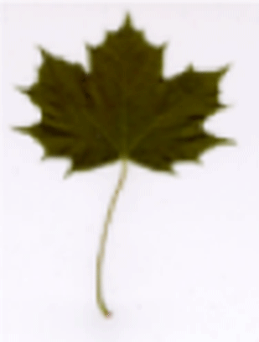
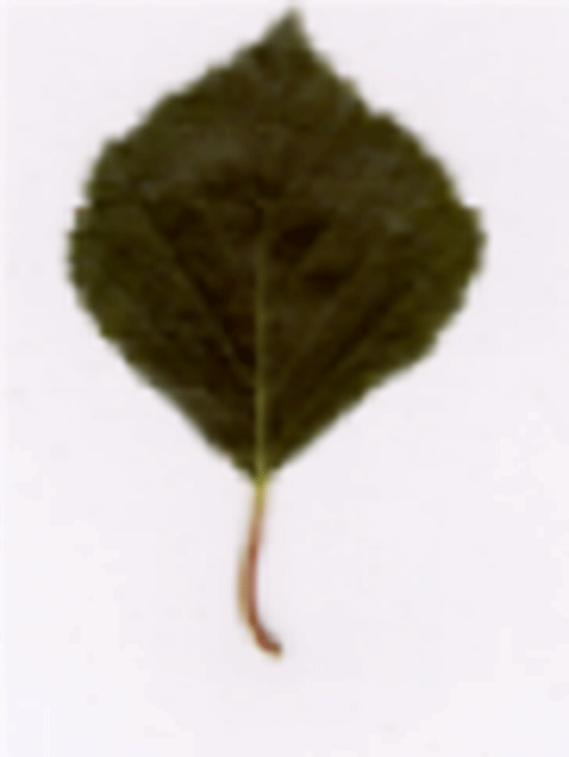
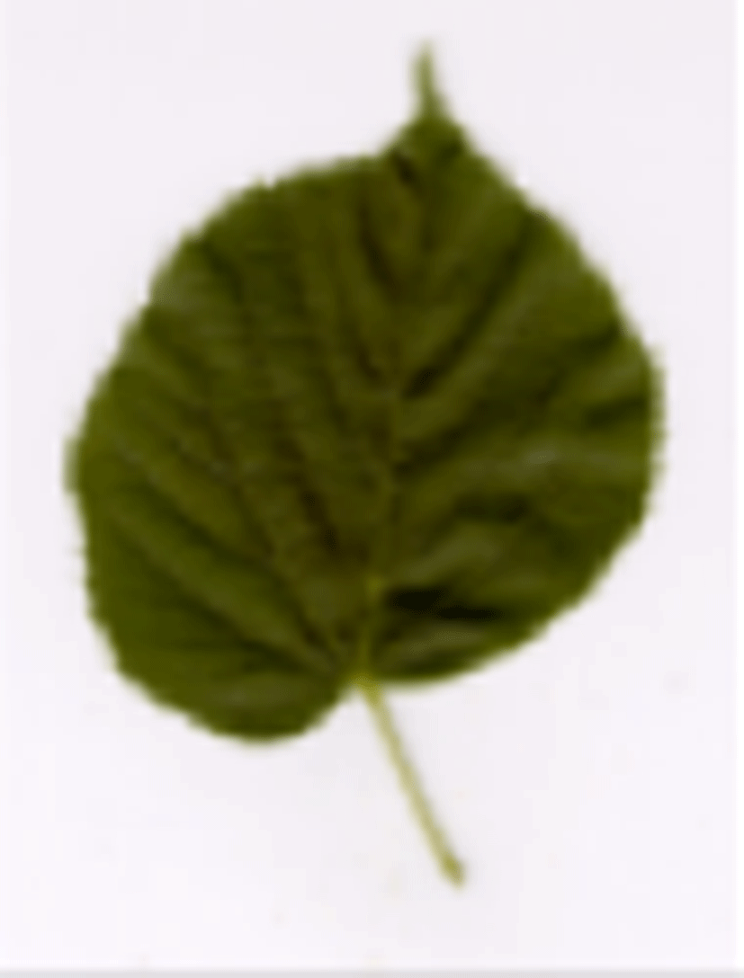
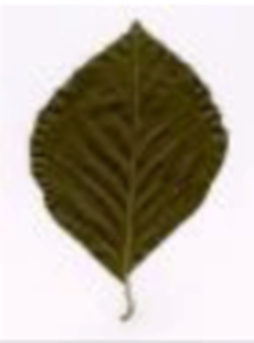
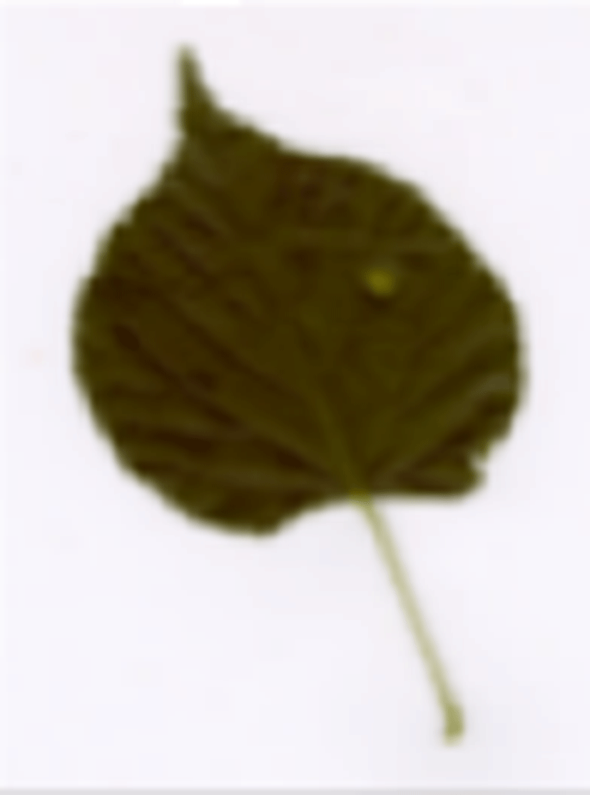
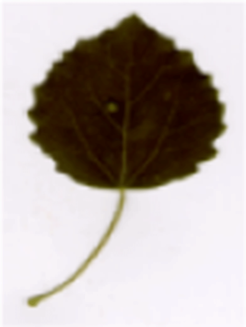
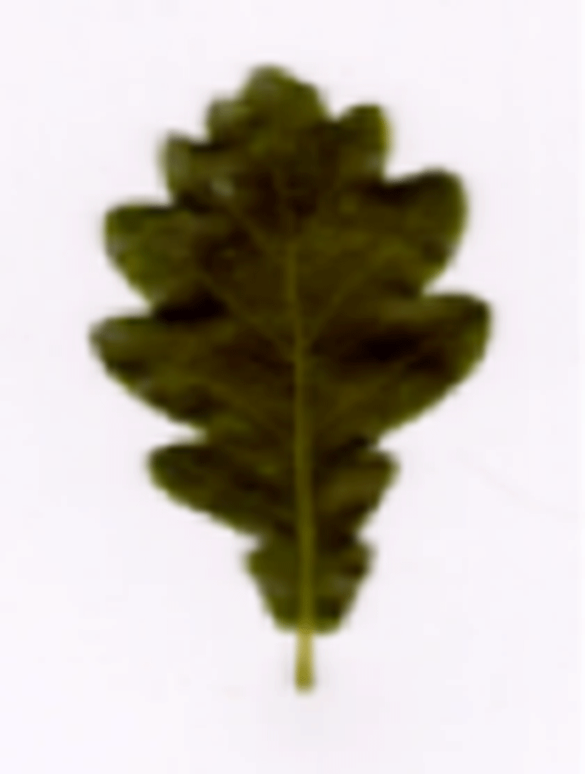
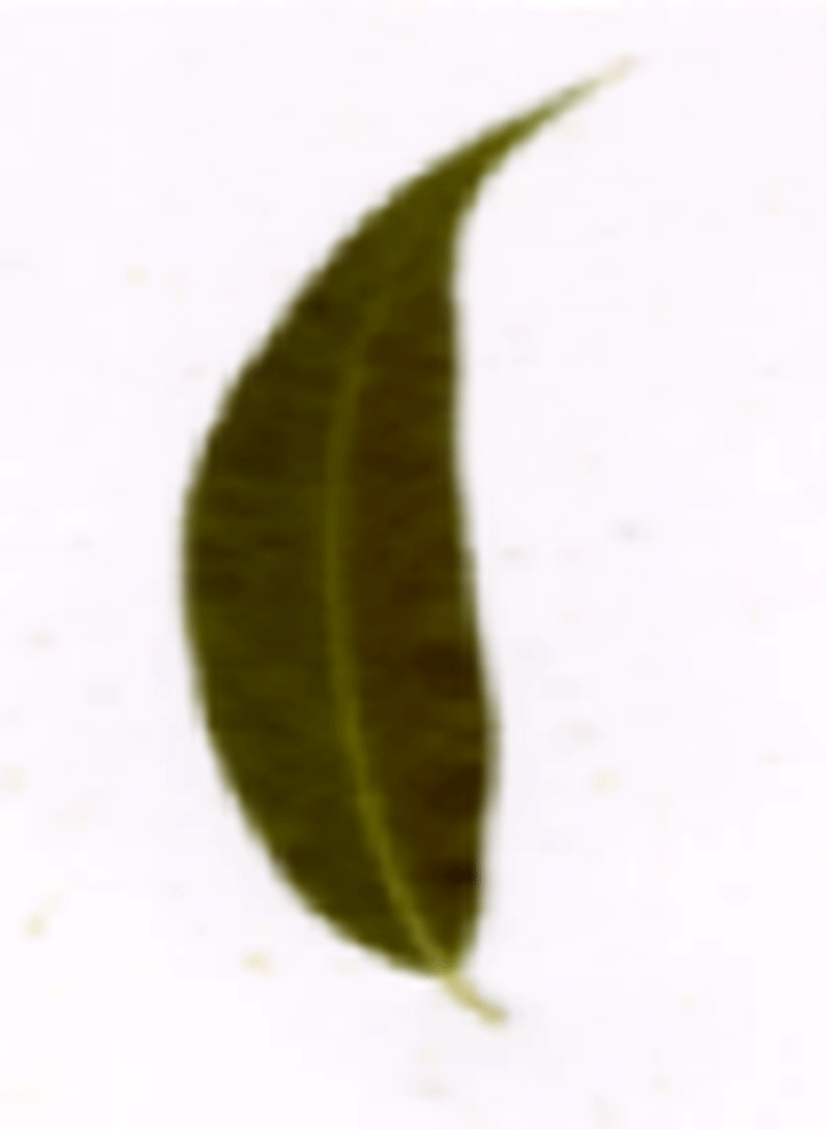
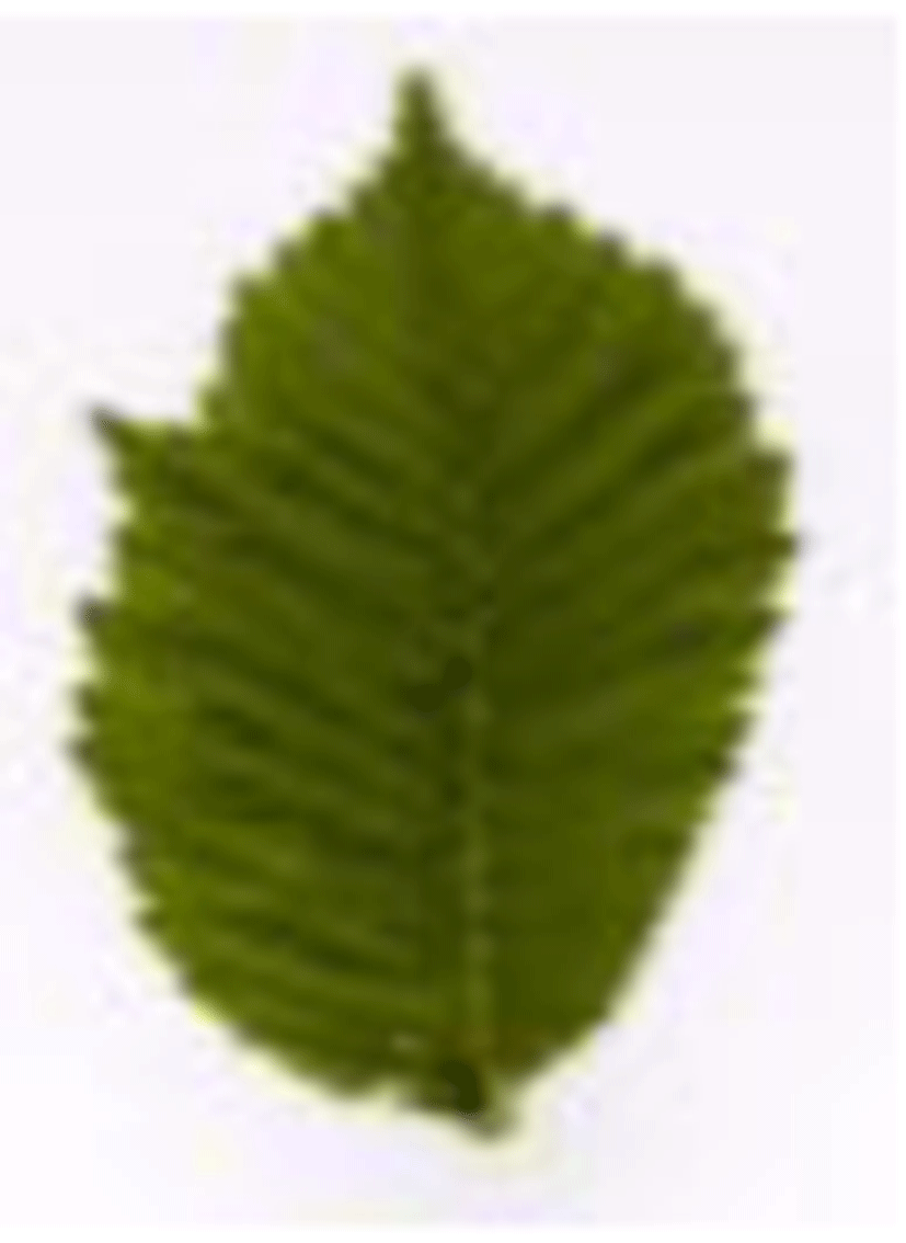
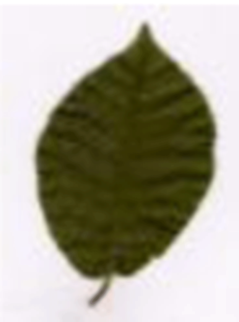
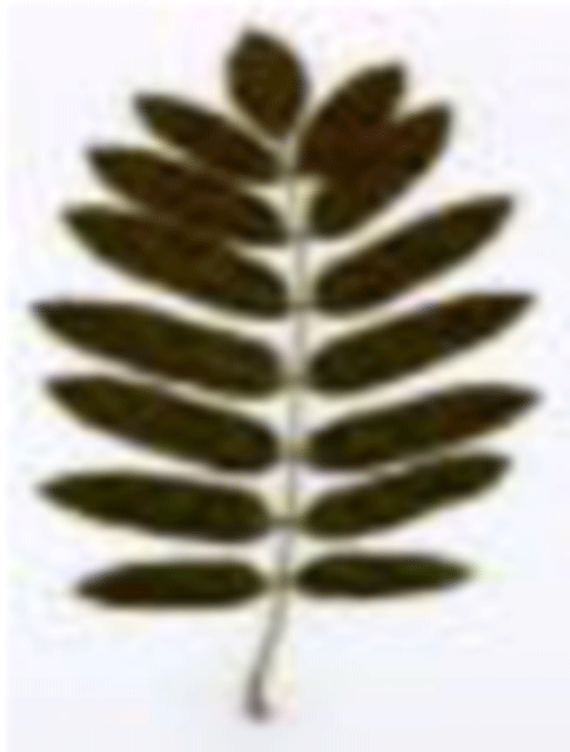
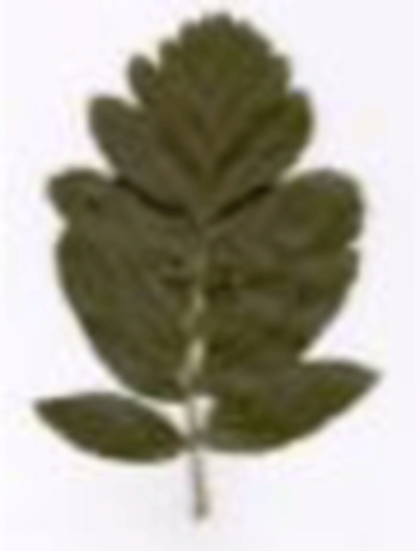
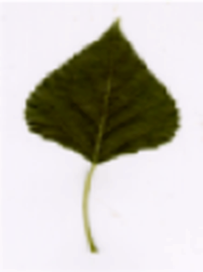
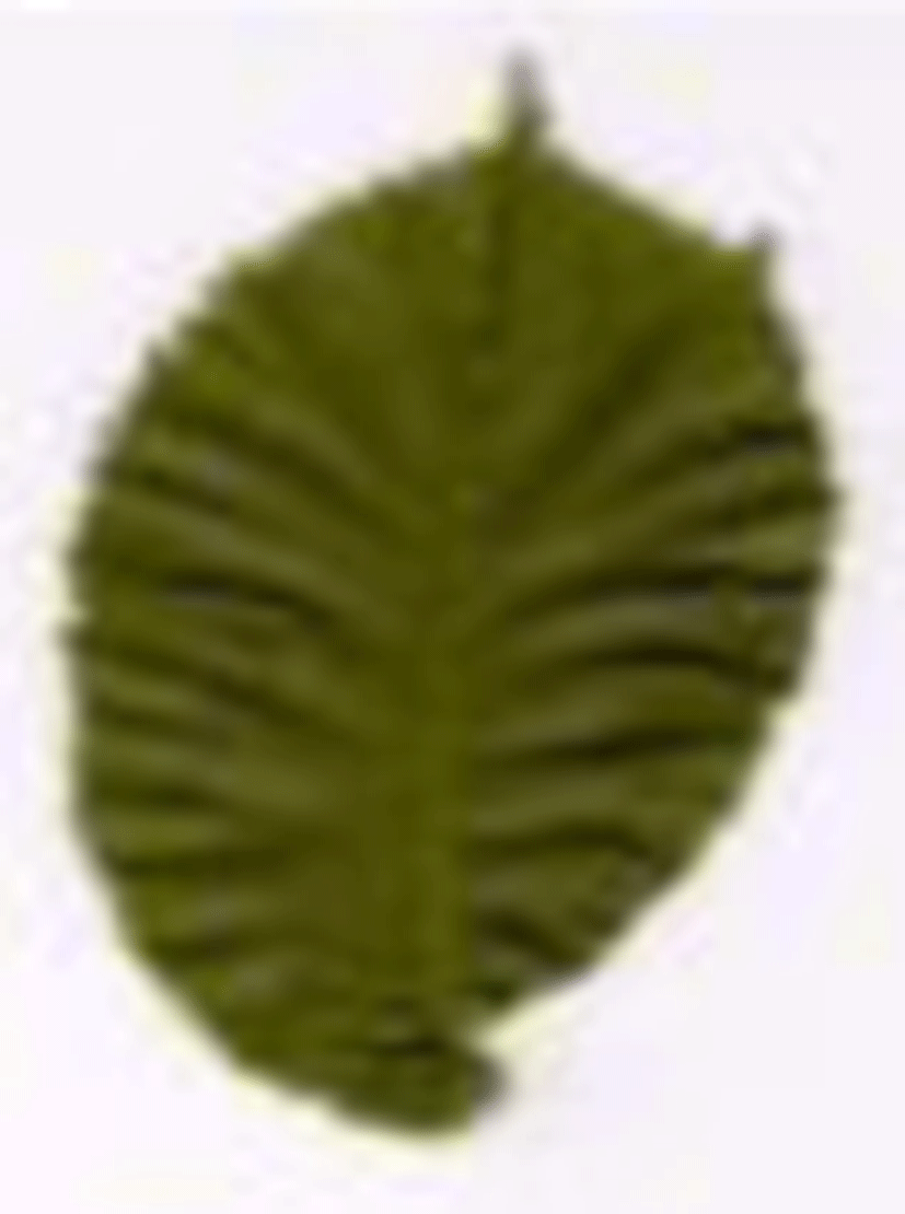
The first step in the process of identification is to acquire the image of the plant. The image taken can be of the entire plant, leaf, flower, stem or even the fruits [2]. Authors in [3] suggest that there are three categories of images based on how the image is acquired, viz. ‘scans’, ‘pseudo-scans’, and ‘photos. In scan and pseudo-scan categories, the leaf images are taken by the method of scanning and photography respectively i.e. the images are captured in front of a plain background indoors. For the third category, the images are of plants are captured in natural environment. Scans and pseudo-scans images are largely used by researchers as they are easy to examine [2]. Typically, the leaves selected are simple, fully grown and not tampered. These are then imaged in the lab under proper lighting conditions. The scans and pseudo-scans simplify the classification task as the image is taken against a plain background. Some of the available standard datasets are Swedish dataset (15 species of leaves), Flavia dataset (32 species of leaves), ICL dataset (220 plant species), etc. Majority studied have worked on images from these three datasets (refer table 1). In our study we have used Swedish dataset [19] which contains 75 images each of 15 species of plants, which makes a total of 1,125 images. The dataset is available in public domain and can be downloaded from the official website (http://www.cvl.isy.liu.se/en/research/datasets/swedish-leaf/). It contains images of plant leaves which are in .tiff format. Table 2 gives the names of the 15 species and one image each from all the species.
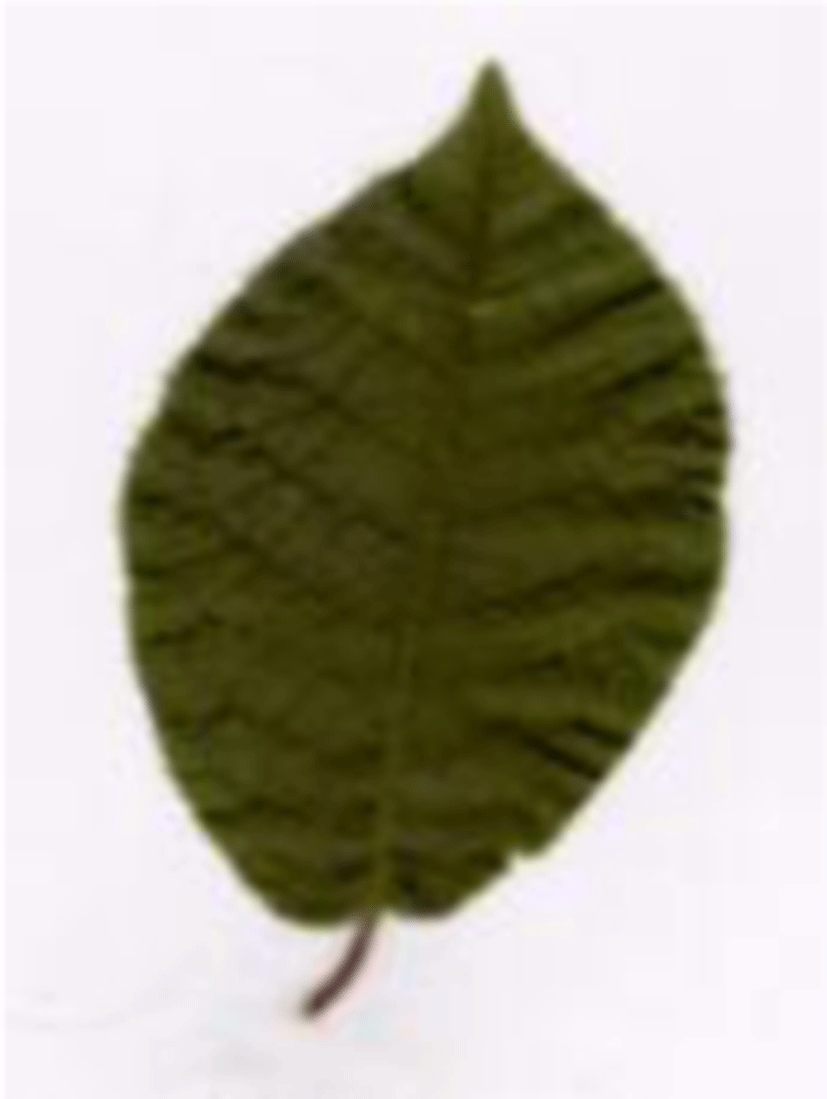
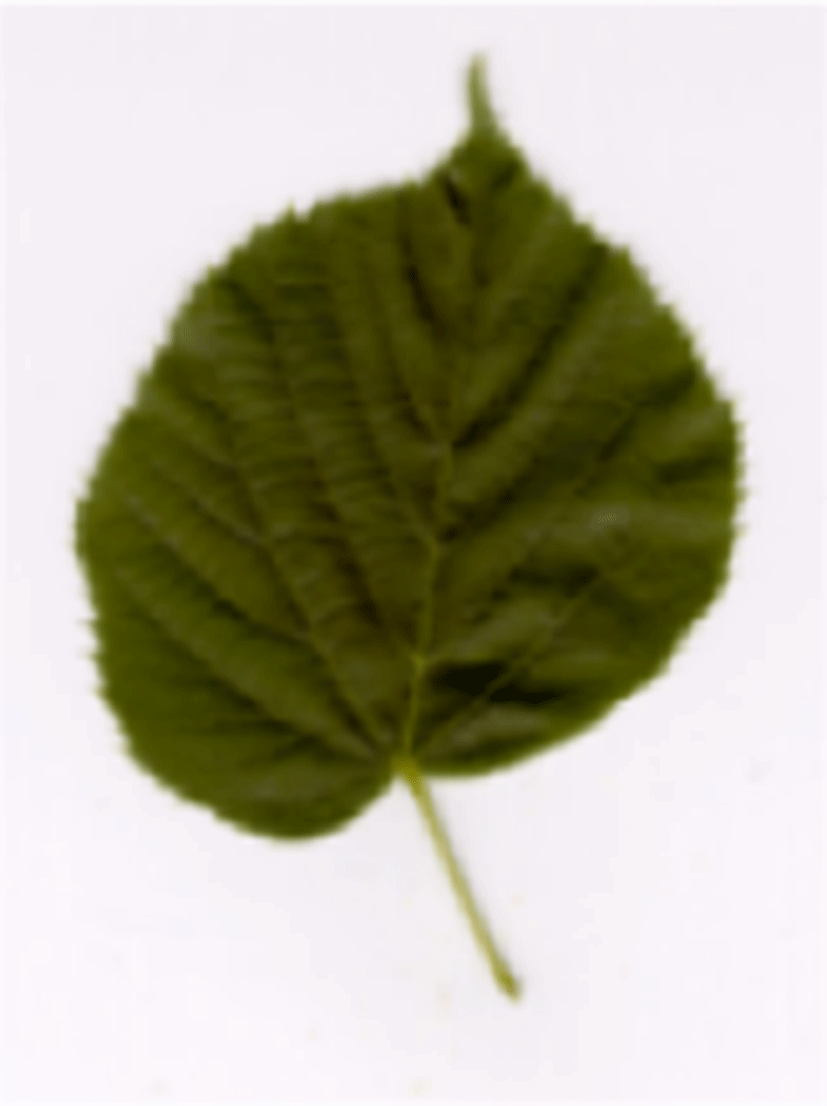
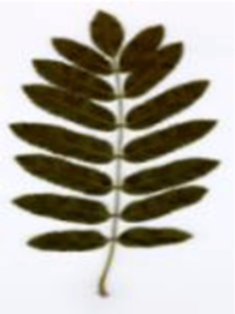
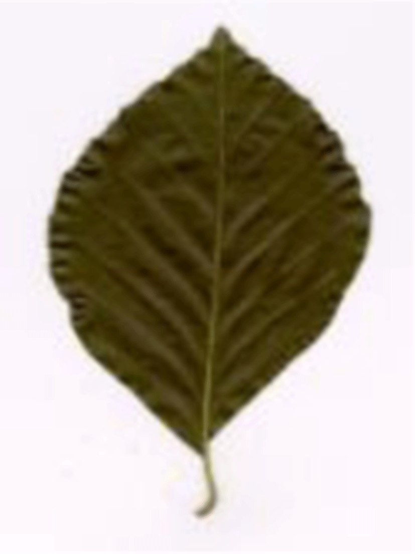
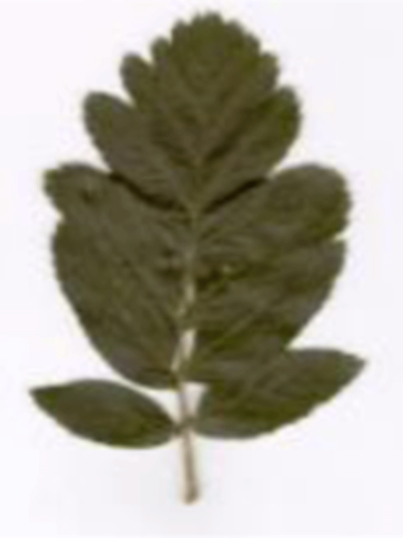
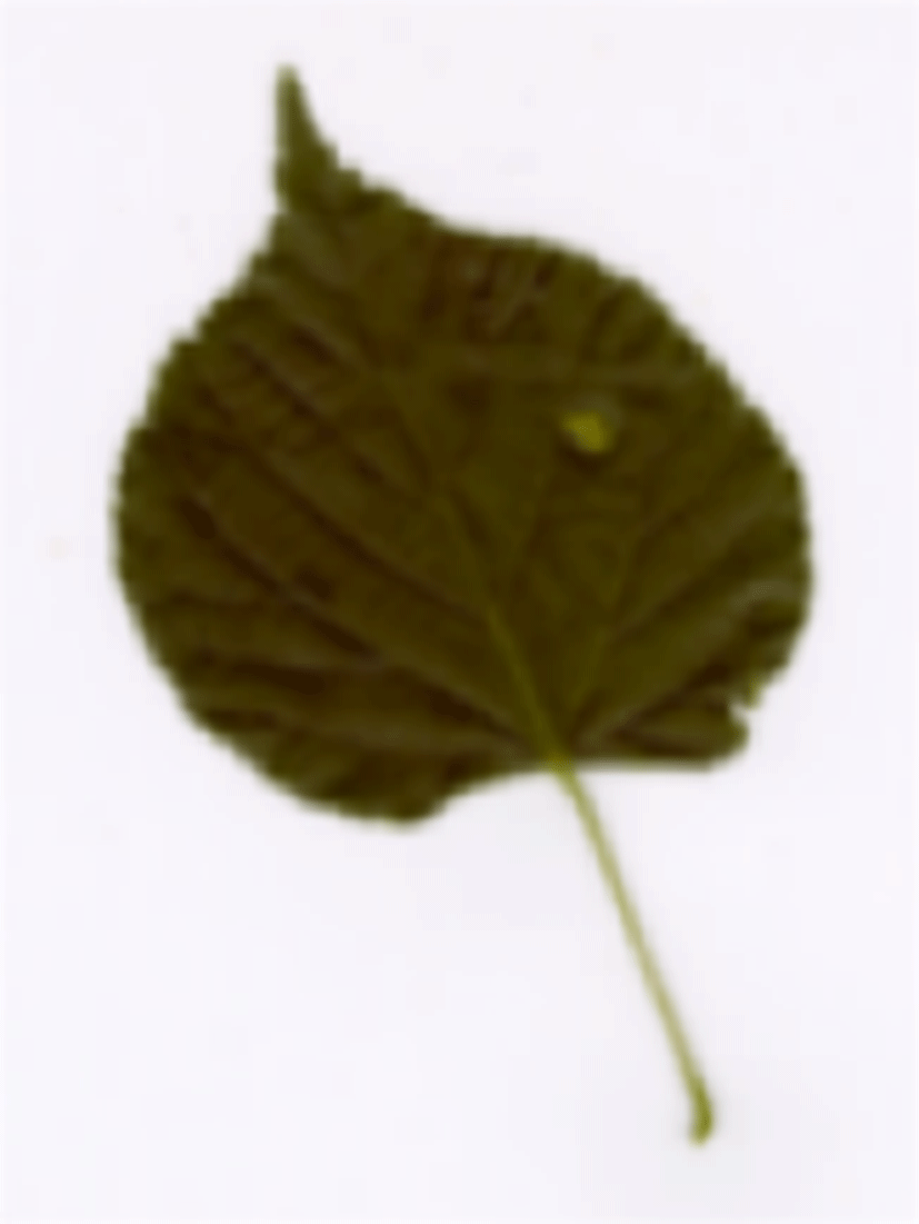
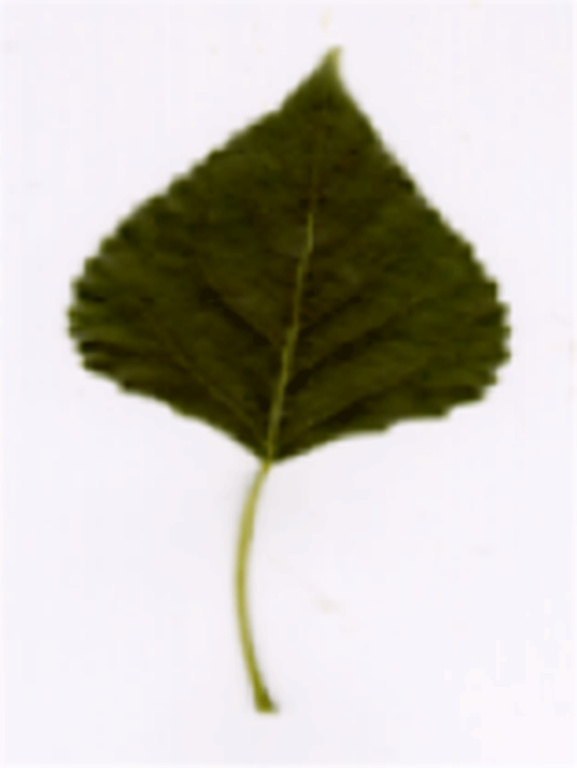
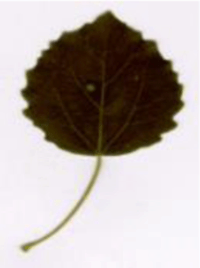

Image pre-processing is an important step as it helps to enhance the quality of image for further processing. This step is necessary as an image inherently contains noise and this may result in lower classification accuracy. It is performed to remove the noise that hampers the identification process and handle the degraded data. A series of operations are followed to improve the image of the leaf which include, converting the RGB image to grayscale, then from grayscale to binary, followed by smoothing, filtering etc [20]. Pre-processing mechanism used in this paper contains noise handling along with resizing operation and image enhancement.
To handle the noise in the images, this study has employed Gaussian Filtering which is also sometimes called Gaussian Smoothing. It is a linear filter which reduces the noise or redundant information in the image. Formula to apply gaussian filter is given in equation 1.
‘α’ is standard deviation, ’a’ is the distance from horizontal axes and ‘b’ is the distance of origin from vertical axes.
After handling noise, resizing operation has been performed. In our study, the images have been resized to [300 × 400]. Resizing is done using equation 2.
Since we are working on color images, image enhancement becomes an essential step to perform. Moreover, the next step involves color image segmentation for which the image contrast and texture needs to be enhanced to obtain better results. Image enhancement removes any redundant pixels present in the color image before performing segmentation [21]. In our study we have enhanced the contrast of the image by contrast stretching which improves the contrast in an image by expanding the dynamic range of intensity values it contains. This step is followed by contrast adjustment which saturates the top one percent and bottom one percent of all pixel values [22]. Figure 2 below shows an enhanced image.
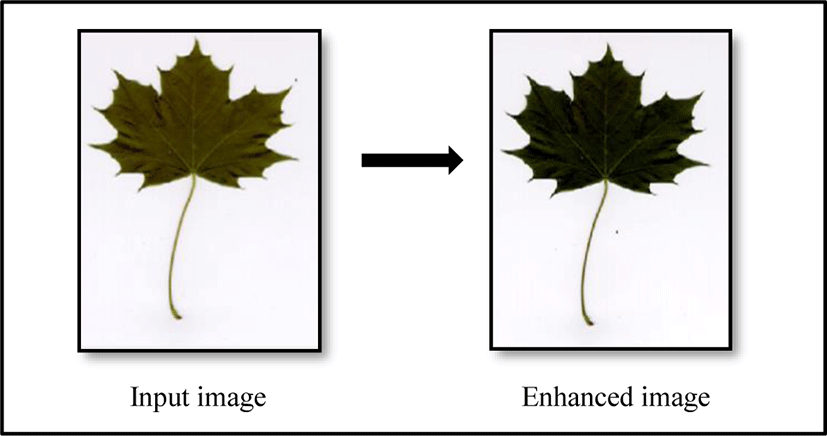
Image segmentation is an important step and critical step for image analysis and is basically performed to extract the region of interest (ROI). It is a process in which each pixel of the image is individually processed and is grouped together with other pixels in the image which share the same attributes and an image divided into various segments is obtained as the output of the segmentation step [23]. In other words, it is process in which each pixel is assigned a label based on certain characteristics and the pixels that share the similar characteristics are grouped together. The images are generally segmented into different parts (or segments) on the basis texture, color, gray level, pixel intensity value etc [24]. Segmentation plays a significant role as partitioning of images into several parts makes image analysis much easier and manageable. Segmentation is widely used in various application areas such as content-based retrieval, object recognition, medicinal imaging etc.
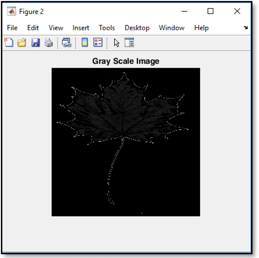
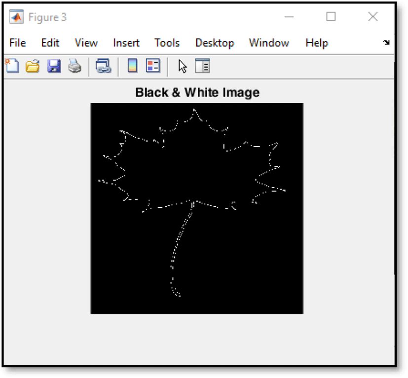
Edge-based method, region-based method, clustering method, watershed method, are some of the segmentation techniques which are widely used in these areas of work. In the past few decades, many studies have performed segmentation on gray-scale images. However, in our study we are dealing with RGB images which require color-based segmentation for further processing of the image. Since color images carry a lot of information within them, thus processing a color image as it is, reduces the efficiency. With the help of image processing toolbox of MATLAB R2018b, we have implemented color based segmentation by applying k-means clustering technique and three different clusters were generated (one each for ‘R’, ‘G’, ‘B’). These three images thus obtained can be used individually for further processing of the input image in the subsequent steps. Figure 3 illustrates an example of the segmentation performed in our system. Out of the three images generated, the selected image is then converted to gray-scale and binary for extraction of certain features which will be discussed in the next section. Figures 4 and 5 illustrate the gray-scale and binary images respectively of the segmented image represented by the caption ‘cluster 2’ in figure 3.

After performing pre-processing and segmenting the image into desired region of interest, feature extraction is performed. It is regarded as one of the most important steps in image processing and pattern analysis. Feature extraction can also be considered dimensionality reduction process. An image inherently contains a lot of information, all of which cannot be processed as it may contain redundant data and such huge amount of data requires large amount of computation power and memory [25]. Hence, feature extraction is performed to reduce the number of variables for further processing of the image. Choosing the right set of features to optimally describe the image thus becomes very important. In our study, we have used a combination of texture and color features to represent the image.
Texture analysis is very significant in many areas such as medical imaging, image retrieval. Texture as a term in image processing defines various properties of images such as smoothness, coarseness, regularity etc. It represents the spatial distribution of the grey-levels of the pixels of a digital image in a neighbourhood.
There are four methods of extracting texture features viz. statistical, structural, model-based and transform-based. In our study, we have used statistical method which characterises texture by the statistical properties of the grey-level image. Statistical methods can be classified as first order (one pixel), second order (two pixels) and higher order (three or more pixels). The first order statistics (or histogram-based features), calculate texture features from the individual pixel irrespective of the relationship of the pixel with its neighbours. Second order statistics take into account the pixels that occur relative to each other [26]. We have used GLCM (Grey-Level Co-occurrence Matrix) for texture feature extraction which is one of the most studied second order statistics. GLCM considers the spatial relation of pixels and extracts texture features by creating a matrix by calculating how often a pixel with grey-level value ‘i’ occurs in a specific spatial relation to grey-level value ‘j’ [27]. In other words, it considers relationship between two pixels at a time called the reference pixel and neighbour pixel. Haralick [28] derived 14 features from GLCM.
We have used five features viz. ‘contrast’, ‘correlation’, ‘energy’, ‘entropy’, and ‘homogeneity’. The formulas of these features are given in table 3 where ‘i’ and ‘j’ are spatial coordinates of the function ‘Pi,j’ , ‘N’ is grey tone and ‘σx’, ‘σy’ represent the standard deviation of x and y coordinates of the image.
| Feature | Formula |
|---|---|
| Contrast | |
| Correlation | |
| Energy | |
| Entropy | |
| Homogeneity |
In the segmentation phase, the input image was divided into three different color channels. Color features are extracted individually from all three images generated as an output of segmentation phase. The color features extracted in this paper can also be referred to as color-based texture features as we have extracted features (mean, S.D., kurtosis, skewness) based on first order statistics from colored image rather than the usual grey-scale. The formulas of these features are given in table 4 where ‘xi’ represents the individual pixel and ‘N’ is the number of pixels.
| Feature | Formula |
|---|---|
| Mean | |
| Standard Deviation (S.D.) | |
| Skewness | |
| Kurtosis |
The above steps have been implemented in MATLAB R2018b environment. The features extracted for an image are then stored in the feature database for subsequent classification of the images to their desired species.
Classification in our work, typically means to assign a certain plant species to the image based on the feature set extracted. In other words, classification is a process of identifying the class label of a new input image on the basis of the prior knowledge (training dataset). For our study, we have used a supervised classification technique in which the labels of the classes (here, plant species) are already known and the new data input is assigned to one of the labels.
Support vector machine is one of the most effective and robust technique used for classification. It incorporates supervised learning techniques which are implemented for classification and regression [29]. SVM was originally developed by Vapnik [30] and has been widely used by researches in the area of image processing [ls] due to its ability to maximise predictive accuracy and tendency to avoid over-fitting of data [31].
Typically, SVM is a binary classifier that classifies data into 2 classes. Classification by SVM is performed by constructing a hyperplane (or set of hyperplanes) in a n-dimensional space (where ‘n’ is the number of features) that distinctly classifies input data points. An optimal hyperplane is the one that achieves maximum margin between positive and negatives classes [16]. SVM classifier is built by employing a kernel function, which transforms the input data into higher dimensional feature space and a hyperplane which optimally separates 2 classes is thus constructed [32]. Since in this study, number of classes (i.e. plant species) are more than two, we have used Multiclass-SVM (MSVM). The MSVMs are generally implemented by combining binary SVMs [33]. The MSVM used in this study implements ‘one-vs-all’ approach in which the ith SVM is trained such that the samples of ith class are specified as ‘positive’ and the rest ‘negative’.
IV. RESULTS
The proposed methodology was tested on Swedish dataset which contains 1,125 images of 15 different species (table 2 gives the names of all the species). The dataset typically contains single leaf images of plants. The leaves are mostly in good shape and fully grown. A very few (almost negligible) leaves are distorted or slightly deformed. The dataset shows high intra-class similarity as well as inter-class similarity in a very few cases.
For this study, the images of the dataset are resized to [300 ×400]. The input image is first processed to remove any inappropriate data or noise contained in the image by filtering and contrast enhancement. This step is necessary since the images in the dataset are colored and an RGB image contains redundant information which need not be processed. Pre-processing, in this study, includes filtering and image enhancement (as shown in figure 2). After pre-processing, the model employs color-based segmentation to segment the image into three clusters by applying k-means clustering technique (result of this step is as shown in figure 3). Feature extraction phase extracts second order GLCM features (‘energy’, ‘entropy’, ‘contrast’, ‘correlation’, ‘homogeneity’) which specify the details about the texture of the leaf image. To make classification more efficient, four color features (‘mean’, ‘standard deviation’, ‘kurtosis’, ‘skewness’) are extracted along with five texture features. Majority of the previous studied have used only shape features [8, 11, 12,15-18] for plant identification. This study however, emphasises on texture and color features because shape features cannot always correctly identify a plant. For instance, while working on plant images taken in natural environment, the leaves can often be damaged or not fully grown. In such cases, shape feature extraction can prove inefficient and unreliable. In the last step of the proposed methodology, the features are used to train the SVM classifier using ‘one-vs-all” approach. Multiclass-SVM was trained using 70% of the images and 30% images were utilised for testing.
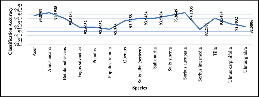
Five images from testing sets of each species were used to test the overall accuracy of the system. Table 5 gives the results of feature extraction for one image each from the testing sets of all the species. The GLCM texture features represent the relationship between a pair of pixels of a gray-scale image: ‘Contrast’ measures the intensity of a pixel and the neighbour pixel over the entre image; ‘Correlation’ represents the similarity between two neighbour pixels; ‘Energy’ depicts the uniformity of the image; ‘Homogeneity’ measures the closeness of the distribution of GLCM elements [26]; ‘Entropy’ is the measure of uncertainty in a gray-scale image. Entropy is generally inversely proportional to energy. For e.g. the image belonging to the species Ulmus glabra has the highest entropy value of 2.06 and the corresponding energy value is the lowest i.e. 0.64. The color features are first order statistics and consider only the individual pixels: Mean is the average of all pixels in the image which can also be termed as average color of the image [34]; Standard Deviation is measure of the deviation or variation from the mean value; Skewness is the degree of asymmetry of the color distribution; Kurtosis specifies the shape of the distribution. The classifier achieved accuracy as high as 94.19% for two classes (Alnus incana and Sorbus aucuparia) and the lowest accuracy obtained was 92.25% for Populus tremula. The system achieved an aggregate accuracy of 93.26%. The accuracy values achieved for individual species are shown in figure 6. Classification accuracy is expressed as given in equation 3:
where TP is True Positive, TN is True Negative, FP is False Positive and FN is False Negative.
V. CONCLUSION
This paper has proposed an automatic plant species identification approach which is employed using computer vision and machine learning techniques to classify plant leaf images. The study has been conducted in phases like image pre-processing, image segmentation, feature extraction and finally classification of the image. A combination of texture and color features (5 and 4 respectively) were extracted and then SVM classifier was used for classification. The system was tested on Swedish dataset and attained an average accuracy of 93.26%. the model could automatically classify 15 different plant species. Texture and color feature space performed satisfactorily well in comparison to the methods which work only on morphological shape features. Also, SVM as a classifier performed considerably well when compared to PNN, k-NN. The proposed method is very easy to implement and efficient. Although the model achieved an accuracy of more than 90%, it still lags in comparison to methods implementing neural networks or deep learning techniques. In future, we aim to overcome this limitation and achieve higher accuracy by extracting much more cultivated features of all types (shape, texture, color and vein) and implementing improved classifier or a hybrid of classifiers. Finally, the objective is to make the idea of automatic plant species identification more realistic by working on live dataset.